Born-Oppenheimer Molecular Dynamics
This tutorial aims at presenting how to perform a Born-Oppenheimer Molecular Dynamics (BOMD) simulation with Octopus, as well as the related tools that can be used to analyze the data generated by such a run. A typical BOMD simulation goes as follows. One first computes the ground state of the system under interest. Then, one performs the actual time evolution, in which the ions are evolved, using a velocity Verlet algorithm, and the electrons remain in their ground state at each step of the time evolution. A SCF cycle is then done for each step of the molecular dynamics, after which the electronic forces are computed.
Ground-state input file
As always, we will start with a simple input file. As an example, in this tutorial we will look at the case of a Water molecule:
CalculationMode = gs
FromScratch = yes

BoxShape = parallelepiped
Lsize = 7

%Coordinates
 'O'  |  0.000000  | -0.553586  |  0.000000
 'H'  |  1.429937  |  0.553586  |  0.000000
 'H'  | -1.429937  |  0.553586  |  0.000000
%

Spacing = 0.5

Eigensolver = chebyshev_filter
ExtraStates = 4
Now run Octopus using the above input file. This produces the usual output, as described in previous tutorials.
From the static/info file, one can find the usual information of the ground-state of the water molecule. As H2O is a polar molecule, we can in particular find the dipole moment of the molecule, which is here of about 1.33 Debye, quite far from the experimental value of 1.855 Debye, see Ref.1, as the calculation is not converged here.
Born-Oppenheimer molecular dynamics
Let us now perform the BOMD calculation. For this, we will use the following input file:
CalculationMode = td
FromScratch = yes

BoxShape = parallelepiped
Lsize = 7

%Coordinates
 'O'  |  0.000000  | -0.553586  |  0.000000
 'H'  |  1.429937  |  0.553586  |  0.000000
 'H'  | -1.429937  |  0.553586  |  0.000000
%

Spacing = 0.5

Eigensolver = chebyshev_filter
ChebyshevFilterNIter = 0
OptimizeChebyshevFilterDegree = no
ExtraStates = 4

TDDynamics = bo
TDTimeStep = 20.0
TDPropagationTime = 50*fs
MoveIons = yes

ParStates = no
In order to perform the BOMD, we changed few thing in the above input file. First, we change the CalculationMode to td, as we are now perforing a time evolution. In order to tell Octopus that we want a BOMD calculation, we set the variable TDDynamics to bo. We further activated the motion of the ions using MoveIons = yes.
In order to make the run fast, we also here deactivated the parallelization over states, using ParStates = no, and tuned some parameters of the Chebyshev filtering to avoid recomputing initial bounds of the filters, as each BOMD step provides a good initial starting point for the next one.
It should be noted that the parameters used in this tutorial (box size, grid spacing, tolerance on the relative density…) are not converged, and should be adjusted for any practical calculation.
Analysis of the results
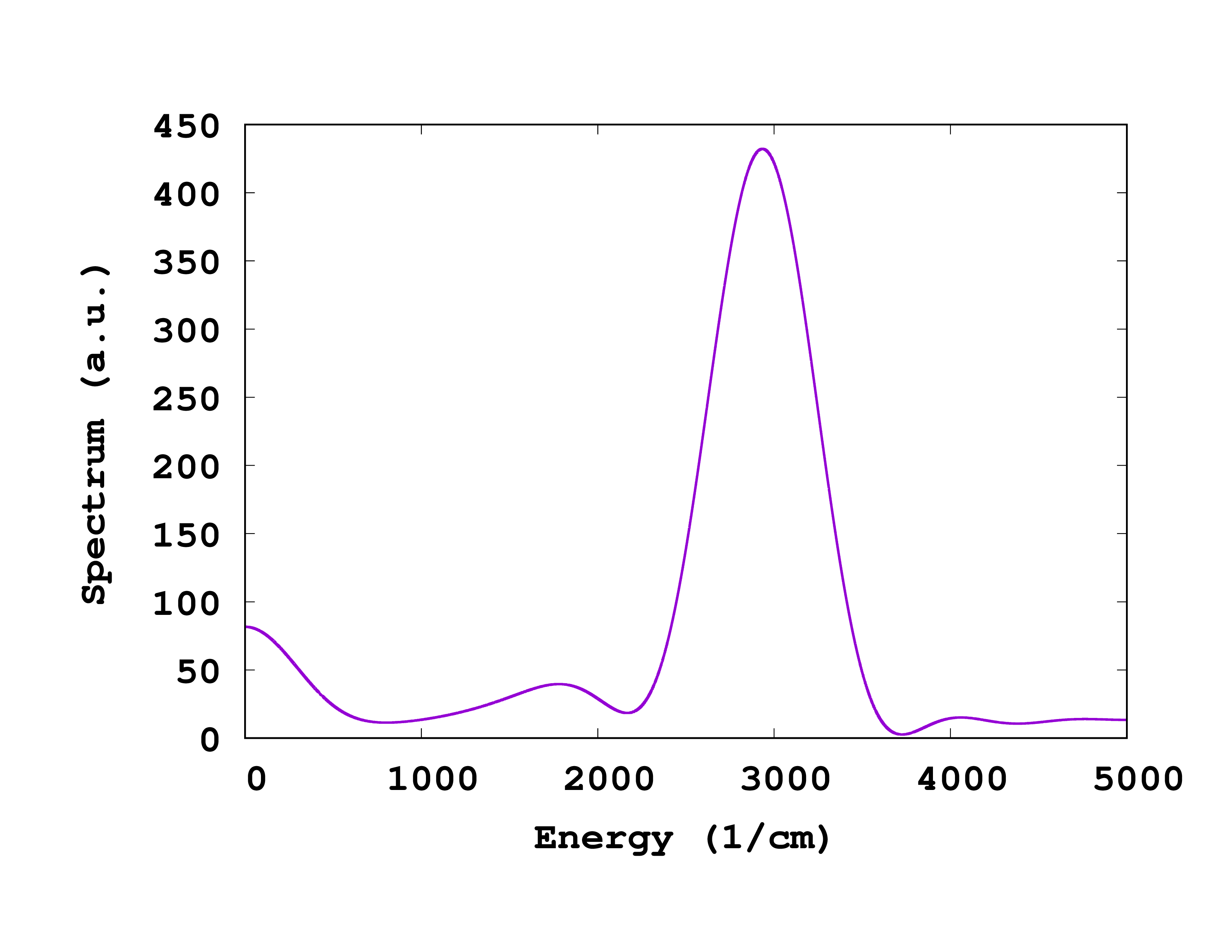
In order to analyze the motion of the molecule, we now compute the velocity correlation function and compute its Fourier transform. This is done using the tool oct-vibrational_spectrum. As we performed here a relatively short calculation, we want to use all the time steps for the analysis, so we use
VibrationalSpectrumTimeStepFactor = 1
After running the utility, we obtain the files td.general/velocity_autocorrelation and td.general/vibrational_spectrum. Plotting the file td.general/vibrational_spectrum shows the spectrum of the velocity correlation function, displaying peaks at the vibrational modes of H2O, see Fig. 1. We observe a main peak around 3000 cm^-1, as well as other side structures.
Generate a movie from the actual data
Let us finally produce a movie from the coordinates generated during the BOMD run. For this, one can use the utility oct-xyz-anim. This generates a file called td.general/movie.xyz, that can be later converted to an animated GIF using for instance XCrysden.
The resulting movie is shown in Fig. 2 below, for a longer simulation of 100fs, using a tighter relative density convergence criterim of 1e-7, and otherwise the same input parameters as the above input. It is possible to use the variable AnimationSampling to select how many frame are used for the movie. In order to produce the movie below, we used AnimationSampling=1.
References
-
Shelley L. Shostak; William L. Ebenstein; J. S. Muenter, The dipole moment of water. I. Dipole moments and hyperfine properties of H2O and HDO in the ground and excited vibrational states, J. Chem. Phys. 94 5875 (1991); ↩︎