Absorbing boundaries

In this tutorial, we explore how to work with absorbing boundaries. For this, we will model the dynamics of an electron wavepacket scattering in a one-dimensional box and see how we can employ absorbing boundaries to efficiently avoid reflection at the edge of the simulation box.

Ground state

We will start with an input file containing only the description of a 1D hydrogen atom, modeled by a soft Coulomb potential. The details of this physical system are not really relevant here, as we will replace the electronic state with a user-defined state for the time-dependent calculation.

FromScratch = yes
CalculationMode = gs

Dimensions = 1

Radius = 50
Spacing = 0.15

%Species
 "H" | species_soft_coulomb | softening | 1 | valence | 1
%

%Coordinates
 "H" | -10
%

SpinComponents = polarized

ExtraStates = 1

%Occupations
 1 | 0
 0 | 0
%

These input variables should already be familiar as they have been explained in previous tutorials. Run Octopus on this input file to get the ground state of the electronic system.

No absorbing boundaries

We are now ready to perform a simulation of the time-evolution of a wave-packet, without absorbing boundaries. For this, we use the following input file:

FromScratch = yes
CalculationMode = td

Dimensions = 1

Radius = 50
Spacing = 0.15

%Species
"H" | species_soft_coulomb | softening | 1 | valence | 1
%

%Coordinates
"H" | -10
%

SpinComponents = polarized

ExtraStates = 1

%Occupations
 1 | 0
 0 | 0
%

a = 0.1
x0 = 10.0
p = 5.
%UserDefinedStates
  1 | 1 | 1 | formula | "exp(-a*(x-x0)^2+i*p*(x-x0))"
%

%Output
 density
 potential
%
OutputFormat = axis_x

TDPropagationTime = 0.5 * femtosecond
TDTimeStep = 0.01

In order to introduce the electron wavepacket to scatter on the hydrogen atom, we have done the following change:

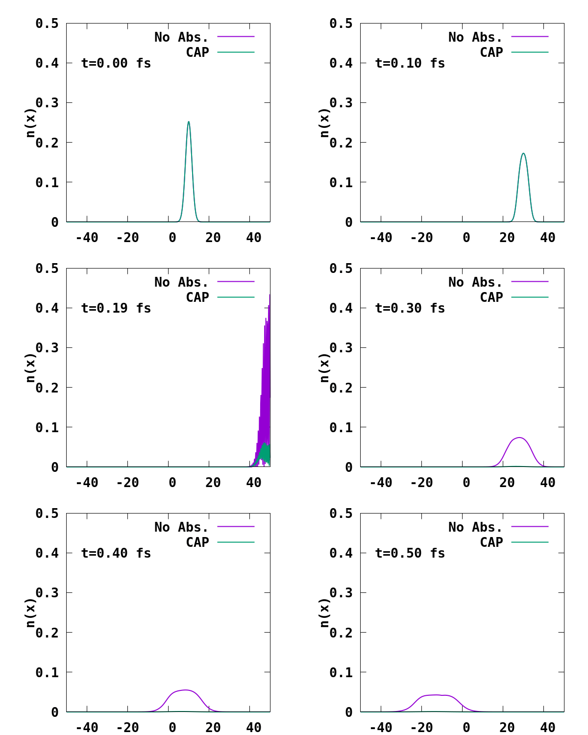
• UserDefinedStates: We are replacing the originally unoccupied state obtained after the GS calculation by a user defined state, which is a Gaussian of the form $ \phi(x) = e^{-\alpha (x-x_0)^2+i p (x-x_0)}, $ where $\alpha$ is taken to be $\alpha=0.1$ here, $x_0=-10$ (a.u.) is the initial position of the wavepacket, and $p$ its velocity, taken to be $p=5$ a.u., such that the wavepacket is sent directly through the hard wall of the simulation box.

Now, run Octopus with this input file, and rename the folder ‘output_iter’ to ‘output_iter_noabs’. We will use these data to compare with the case with absorbing boundaries.

Let us now include the absorbing boundaries. While Octopus provides several methods, we will use the complex absorbing potential (CAP) method. This is done by adding:

  AbsorbingBoundaries = cap
  ABCapHeight = -1
  %ABShape
   40 | 50 | "abs(x)"
  %

The variable AbsorbingBoundaries selects the type of absorbing boundaries. The height of the complex potential is controlled by ABCapHeight, and ABShape allows specification of the shape. Here we are absorbing in the region $40<|x|<50$. In practice, the height of the complex potential, as well as the width of the absorbing region, need to be selected with care, as the reflection error (i.e. how much of the wavepack is not absorbed) is determined by these parameters. More details can be found in the implementation paper.

The result of the calculation is shown in Fig. 1. Without absorbing boundaries, we observe an artificial reflection of the electron wavepacket at the border of the simulation box, which would cause a problem if we were interested in the electron dynamics inside our simulation box. As expected, this is fixed by using absorbing boundaries, which efficiently damp the out-going wavepacket, avoiding the use of extremely large simulation boxes, which are numerically very expensive.

Gnuplot script

In order to produce the above movie, one can use the following gnuplot script

set terminal pngcairo font "Monospace-Bold,20" size 600,500

do for [t=0:2050:50] {

 set output sprintf('density_%04i.png',t)

 set xrange [-50:50]
 set yrange [0:0.5]

 set tmargin 1.5
 set bmargin 1.5

 set xlabel "x [Bohr]" offset 0.0, 0.5
 set ylabel "n(x)" offset 2.0,0

 au2fs = 0.024189
 dt = 0.01;

 set label sprintf('t=%.2f fs', t*dt*au2fs) at -43,0.40
 plot sprintf('output_iter_noabs/td.%07i/density-sp1.y=0,z=0', t) u 1:2 w l lw 2 t "No Abs.", \
      sprintf('output_iter/td.%07i/density-sp1.y=0,z=0', t) u 1:2 w l lw 2 t 'CAP'

 unset label
}

and convert it to a movie using convert

convert -delay 30 -loop 0 density_*.png reflection.gif