RDMFT
In this tutorial, you will learn how to do a Reduced Density Matrix Functional Theory (RDMFT) calculation with Octopus.
In contrast to density functional theory or Hartree-Fock theory, here we do not try to find one optimal slater-determinant (single-reference) to describe the ground-state of a given many-body system, but instead approximate the one-body reduced density matrix (1RDM) of the system. Thus, the outcome of an RDMFT minimization is a set of eigen-vectors, so called ‘’natural orbitals’’ (NOs,) and eigenvalues, so-called ‘’natural occupation numbers’’ (NONs), of the 1RDM. One important aspect of this is that we need to use ‘‘more’’ orbitals than the number of electrons. This additional freedom allows to include static correlation in the description of the systems and hence, we can describe settings or processes that are very difficult for single-reference methods. One such process is the ‘‘‘dissociation of a molecule’’’, which we utilize as example for this tutorial: You will learn how to do a properly converged dissociation study of H$_2$. For further information about RDMFT, we can recommend e.g. chapter ‘‘Reduced Density Matrix Functional Theory (RDMFT) and Linear Response Time-Dependent RDMFT (TD-RDMFT)’’ in the book of Ferre, N., Filatov, M. & Huix-Rotllant, M. ‘‘Density-Functional Methods for Excited States’’ (Springer, 2015). doi:10.1007/978-3-319-22081-9
Basic Steps of an RDMFT Calculation
Create the basis
The first thing to notice for RDMFT calculations is that, we will explicitly make use of a ‘‘basis set’’, which is in contrast to the minimization over the full real-space grid that is performed normally with Octopus. Consequently, we always need to do a preliminary calculation to generate our basis set. We will exemplify this for the hydrogen molecule in equilibrium position. Create the following inp file:
CalculationMode = gs
TheoryLevel = independent_particles

Dimensions = 3
Radius = 8
Spacing = 0.15

# distance between H atoms
d = 1.4172 # (equilibrium bond length H2)

%Coordinates
 'H' | 0 | 0 | -d/2
 'H' | 0 | 0 | d/2
%

Eigensolver = Chebyshev_filter

ExtraStates = 14
You should be already familiar with all these variables, so there is no need to explain them again, but we want to stress the two important points here:
- We chose TheoryLevel = independent_particles, which you should always use as a basis in an RDMFT calculation (see actual octopus paper?)
- We set the ExtraStates variable, which controls the size of the basis set that will be used in the RDMFT calculation. Thus in RDMFT, we have with the ‘‘basis set’’ a ‘’new numerical parameter’’ besides the Radius and the Spacing that needs to be converged for a successful calculation. The size of the basis set M is just the number of the orbitals for the ground state (number of electrons divided by 2) plus the number of extra states.
- All the numerical parameters ‘‘depend on each other’’: If we want to include many ExtraStates to have a sufficiently large basis, we will need also a larger Radius and especially a smaller Spacing at a certain point. The reason is that the additional states will have function values bigger than zero in a larger region than the bound states. Additionally, all states are orthogonal to each other, and thus the grid needs to resolve more nodes with an increasing number of ExtraStates.
Perform the RDMFT calculation
With this basis, we can now do our first rdmft calculation. For that, you just need to change the TheoryLevel to ‘rdmft’ and ‘‘add the part ExperimentalFeatures = yes’’. In the standard out there will be some new information:
- Calculating Coulomb and exchange matrix elements in basis –this may take a while–
- Occupation numbers: they are not zero or one/two here but instead fractional!
Natural occupation numbers:
 #st       Occupation
   1   1.934202755548
   2   0.032593322343
   3   0.013705991480
   4   0.008316364168
   5   0.008473676488
   6   0.000689289923
   7   0.000435423074
   8   0.000211681220
   9   0.000221720956
  10   0.000339136476
  11   0.000329368361
  12   0.000185246999
  13   0.000186709648
  14   0.000089074528
  15   0.000020165490
- ‘‘anything else important?’’
Basis Set Convergence
Now, we need to converge our calculation for the three numerical parameters. This needs to be done in some iterative way, which means we first set ExtraStates and then do convergence series for Radius and Spacing as we know it. Then, we utilize the converged values and perform a series for ExtraStates. Having converged ExtraStates, we start again with the series for Radius and Spacing and see if the energy (or better the electron density) still changes considerably. If yes, this meas that the higher lying ExtraStates where net well captured by the simulation box and we need to adjust the parameters again. We go on like this until convergence of all parameters. This sound like a lot of work, but don’t worry, if you have done such convergence studies a few times, you will get a feeling for good values.
So let us do one iteration as example. We start with a guess for ExtraStates, which should not be too small, say 14 (thus $M=1+14=15$) and converge Radius and Spacing. To save time, we did this for you and found the values Radius = 8 Spacing = 0.15. If you feel insecure with such convergence studies, you should have a look in the corresponding tutorial: [[Tutorial:Total_energy_convergence]]
Now let us perform a basis-set series. For that, we first create reference basis by repeating the above calculation with say ExtraStates = 29. We copy the restart folder in a new folder that is called ‘basis’ and execute the following script (if you rename anything you need to change the respective part in the script):
#!/bin/bash

series=ES-series
outfile="$series.dat"
echo "#ES    Energy    1. NON  2.NON" > $outfile
list="4 9 14 19 24 29"

export OCT_PARSE_ENV=1
for param in $list
do
  folder="$series-$param"
  out_tmp=out-RDMFT-$param

  export OCT_EXTRASTATES=${param}

  export OCT_THEORYLEVEL="independent_particles"
  mpirun -n 4 octopus

  export OCT_THEORYLEVEL="rdmft"
  mpirun -n 4 octopus |tee ${out_tmp}

  energy=`grep -a "Total energy" $out_tmp  | tail -1 | awk '{print $3}'`
  seigen=`grep -a " 1  " static/info |  awk '{print $2}'`
  peigen=`grep -a " 2  " static/info |  awk '{print $2}'`
  echo $param $energy $seigen $peigen >> $outfile
done
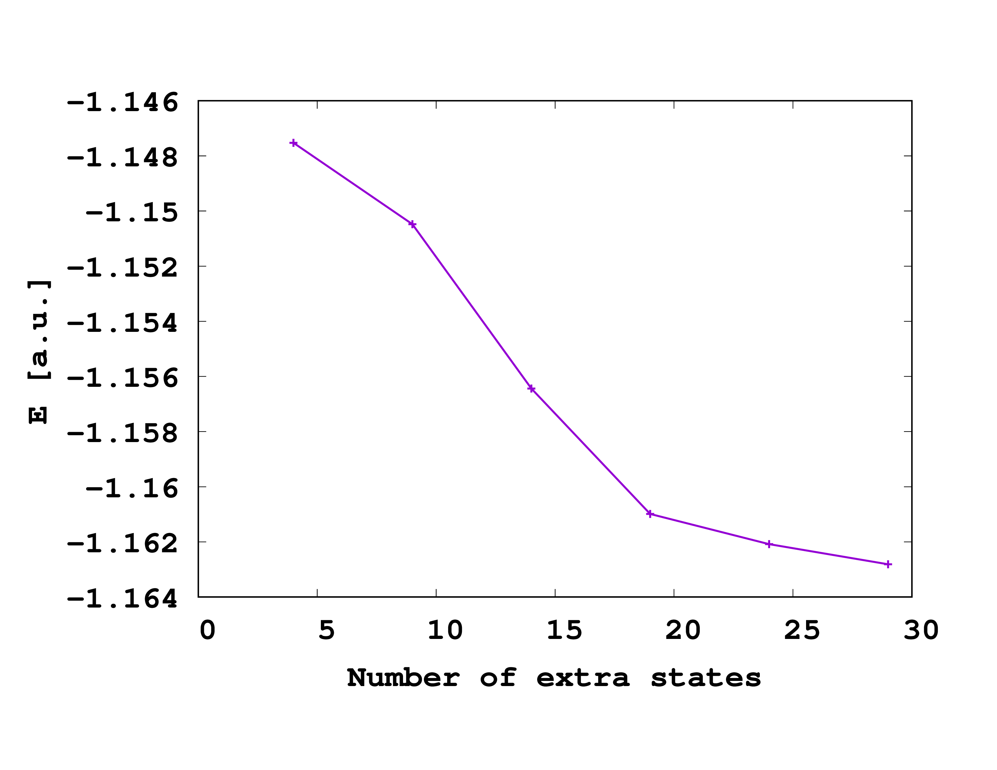
If everything works out fine, you should find the following output in the ‘ES-series.log’ file:
#ES    Energy    1. NON  2.NON
4 -1.1475245557E+00 1.935830015598 0.032403688557
9 -1.1504774505E+00 1.933667143866 0.032143880582
14 -1.1564358980E+00 1.933862324905 0.032368328273
19 -1.1609858740E+00 1.934383717214 0.032654497640
24 -1.1620832131E+00 1.933106604242 0.032855395615
29 -1.1628122033E+00 1.932162093428 0.032941503480

So we see that even with M=30, the calculation is not entirely converged! Thus for a correctly converged result, one would need to further increase the basis and optimize the simulation box. Since the calculations become quite expensive, we would need to do them on a high-performance cluster, which goes beyond the scope of this tutorial. We will thus have to proceed with ‘‘’not entirely converged’’’ parameters in the next section.
H2 Dissociation
In this third and last part of the tutorial, we come back to our original goal: the calculation of the H2 dissociation curve. Now, we want to change the ‘’d’’-parameter in the input file and consequently, we should use an adapted simulation box. Most suited for a dissociation, is the BoxShape= cylinder. However, since this makes the calculations again much more expensive, we just stick to the default choice of BoxShape=minimal .
We choose ExtraStates=14 as a compromise between accuracy and numerical cost and do the d-series with the following script:
#!/bin/bash

series=DIST-series
outfile="$series.dat"
echo "#Dist    Energy    1. NON  2.NON" > $outfile
list="0.25 0.5 0.75 1.0 1.5 2.0 2.5 3.0 4.0 5.0 6.0 8.0"


export OCT_PARSE_ENV=1

for param in $list
do
  echo $param
  folder="$series-$param"
  out_tmp=out-RDMFT-$param

  sed "{s/DISTANCE/$param/g}" inp_template > inp
  rm -rf restart

  export OCT_THEORYLEVEL="independent_particles"
  mpirun -n 8 octopus
  export OCT_THEORYLEVEL="rdmft"
  mpirun -n 8 octopus |tee ${out_tmp}

  energy=`grep -a "Total energy" $out_tmp  | tail -1 | awk '{print $3}'`
  seigen=`grep -a " 1  " static/info |  awk '{print $2}'`
  peigen=`grep -a " 2  " static/info |  awk '{print $2}'`
  echo $param $energy $seigen $peigen >> $outfile
done
The execution of the script should take about 30-60 minutes on a normal machine, so now it’s time for well-deserved coffee!
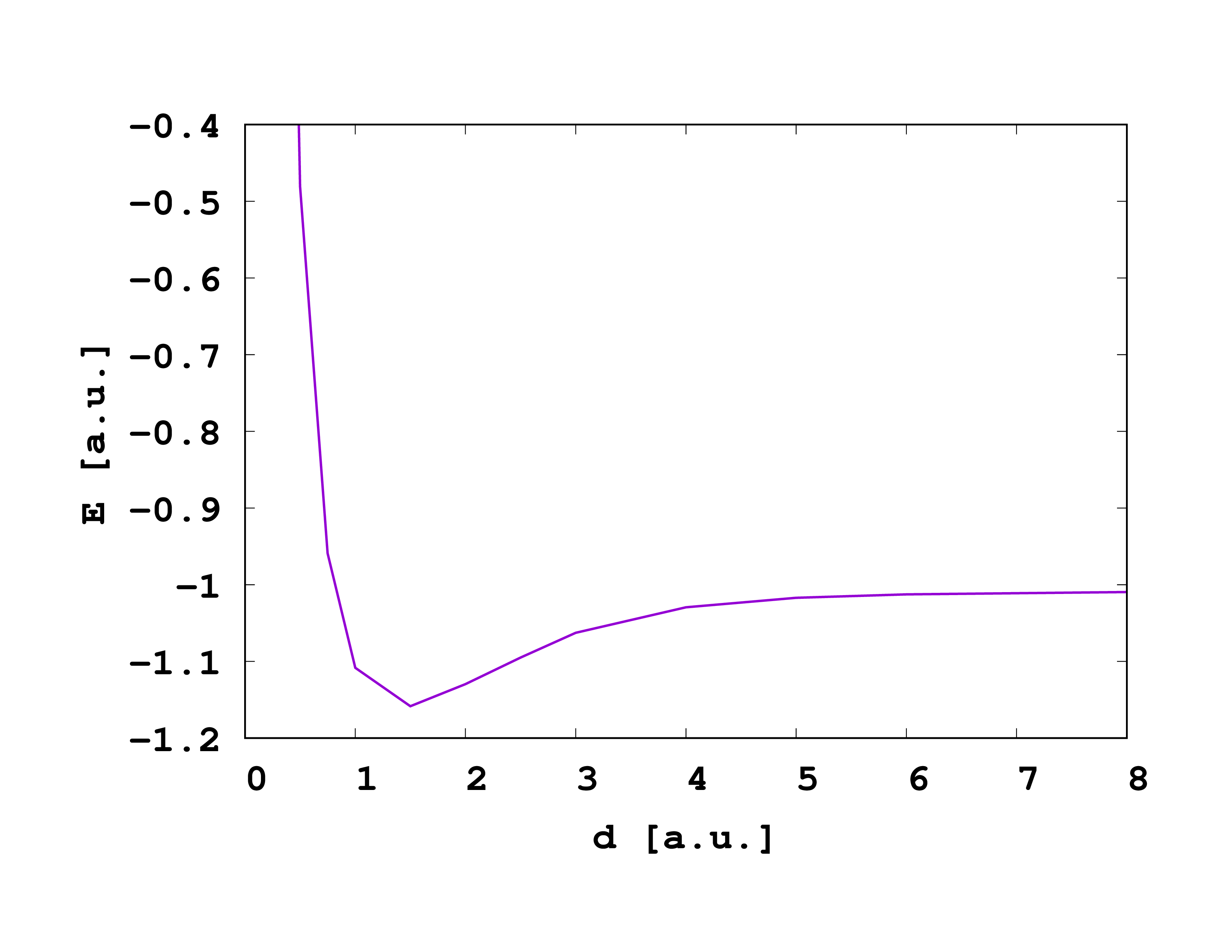
After the script has finished, you have find a new log file and if you plot the energy of the files, you should get something of the following shape:

Comments:
- This dissociation limit is not correct. Since the basis set is not converged, we get a too large value of E_diss=-1.009 than the Müller functional obtains for a converged set (E_diss=-1.047 Hartree), which is paradoxically closer to the exact dissociation limit of E_diss=1.0 Hartree because of an error cancellation (too small bases always increase the energy).
- The principal shape is good. Especially, we see that the curve becomes constant for large d, which single-reference methods cannot reproduce.