Transient absorption
The objective of this tutorial is to give a basic idea of how to perform simulations of transient absorption with Octopus. The transient absorption is an extension of the usual absorption spectroscopy, in which we compute how much a system absorb light when it is brought out of equilibrium by a pump laser.
In order to compute the transient absorption, we need to proceed in three steps. First we need to determine the ground state of the system of interest. In order to make the calculations fast enough, this tutorial uses a periodic model 1D chain of hydrogen dimers. Then, we will compute how the system reacts to the pump laser only. Finally, we will probe the system at different time delays, in order to compute how the system absorbs light out of equilibrium.
Note: This requires to perform one time-dependent simulation for each time delay and can therefore represent an impressive numerical effort if one time evolution of the considered system is numerically expensive.
Ground-state input file
As always, we will start with a simple input file. In this example, we consider a one-dimensional peridoic system with a unit cell composed of an hydrogen dimer.
CalculationMode = gs
Dimensions = 1
PeriodicDimensions = 1
FromScratch = yes

%Species
"Hydrogen1D" | species_soft_coulomb | softening | 1 | valence | 1
%

ll = 1.6
%Coordinates
"Hydrogen1D" | -ll/2
"Hydrogen1D" |  ll/2
%

BoxShape = parallelepiped

%LatticeParameters
 3.6
%

Spacing = 0.5

%KPointsGrid
 100
%

ExtraStates = 5

%KPointsPath
 20
 -0.5
  0.5
%
Now run Octopus using the above input file. This produces the usual output, as described in the previous tutorials.
Pump-only reference calculation
We now start to investigate how our system react to light. For this, we first compute the electronic current that results from the sole pump laser. This will be used as a reference for pump+probe calculations.
For this tutorial, we consider a pump laser with an intensity of 10^10 W.cm^-2, a wavelength of 3200nm, and a duration of 4 cycles. The envelope is taken as a sin-square envelope. As we will need to compute the difference between the pump-probe current and the pump-only current, we need here to specify the total_current as TDOutput.
CalculationMode = td
Dimensions = 1
PeriodicDimensions = 1
FromScratch = yes

%Species
"Hydrogen1D" | species_soft_coulomb | softening | 1 | valence | 1
%

ll = 1.6
%Coordinates
"Hydrogen1D" | -ll/2
"Hydrogen1D" |  ll/2
%

BoxShape = parallelepiped

%LatticeParameters
 3.6
%

Spacing = 0.5

%KPointsGrid
 100
%

ExtraStates = 0

electric_amplitude = (sqrt(10^10)/sqrt(3.509470*10^16))
# Frequency corresponding to 3200nm.
omega = 0.0141375
period = 2*pi/omega
stime = 4*period

%TDExternalFields
 vector_potential | 1.0 | 0.0 | 0.0 | omega | "envelope_function"
%

%TDFunctions
"envelope_function" | tdf_from_expr | "electric_amplitude/omega*c*(sin(pi/stime*t))^2*step(stime-t)"
%

%TDOutput
 total_current
%


TDTimeStep = 1.0
TDPropagator = aetrs
TDPropagationTime = 800 + stime
TDExponentialMethod = lanczos
TDExpOrder = 16
When preparing the reference calculation for performing transient absorption calculation, one needs to decide before what is the energy resolution desired for the transient absorption spectra. In this tutorial, we aim at a broadening of 0.2 eV, which is the energy resolution that one would obtain for a propagation of 800 atomic units. Hence, if we would perform an usual absorption spectrum calculation, we would do a single calculation with a maximum time of 800 atomic units. Here, we want to propagate our system up to a delay time, which if the time at which we want to probe our system. The pump-probe simulations (next section) will then be performed for a maximum time of delay + 800 atomic units.
In order to prepare one pump-only reference calculation, we thus do here a time evolution with a maximum time of the duration of the pulse, plus 800 a.u.. This allows to later explore time delays over then entire duration of the pump laser pulse.
Once the calculation is finished, rename the folder td.general to td.general_ref .
Pump-probe calculations
We will now perform a series of pump-probe calculations, varying the delay at which we apply a kick, as done in the first part of the tutorial Optical spectra of solid.
The prototypical input file is given here:
CalculationMode = td
Dimensions = 1
PeriodicDimensions = 1
FromScratch = yes

%Species
"Hydrogen1D" | species_soft_coulomb | softening | 1 | valence | 1
%

ll = 1.6
%Coordinates
"Hydrogen1D" | -ll/2
"Hydrogen1D" |  ll/2
%

BoxShape = parallelepiped

%LatticeParameters
 3.6
%

Spacing = 0.5

%KPointsGrid
 100
%

ExtraStates = 0

electric_amplitude = (sqrt(10^10)/sqrt(3.509470*10^16))
# Frequency corresponding to 3200nm.
omega = 0.0141375
period = 2*pi/omega
stime = 4*period

delay = DELAY

%TDExternalFields
 vector_potential | 1.0 | 0.0 | 0.0 | omega | "envelope_function"
 vector_potential | 1.0 | 0.0 | 0.0 | 0 | "envelope_step"
%

%TDFunctions
"envelope_function" | tdf_from_expr | "electric_amplitude/omega*c*(sin(pi/stime*t))^2*step(stime-t)"
 "envelope_step" | tdf_from_expr | "0.01*step(t-delay)"
%

%TDOutput
 total_current
%


TDTimeStep = 1.0
TDPropagator = aetrs
TDPropagationTime = 800 + delay
TDExponentialMethod = lanczos
TDExpOrder = 16

ExperimentalFeatures = yes
GaugeFieldDelay = delay
TransientAbsorptionReference = "td.general_ref"

PropagationSpectrumDampMode = gaussian
PropagationSpectrumMaxEnergy  = 5*eV
In order to simplify the calculation of the multiple calculations, one can define a script that takes the above template input file and automatically replaces “DELAY” by the current value, run Octopus, then run the utility oct-conductivity , and move the results into a folder name td.general_delayX , where X is the current delay.
#!/usr/bin/env perl

$delay = 0;
$delaymax = 1500;
$incr = 50;

`rm -r td.general_delay*`;

do{
  print("TD propagation for a delay of $delay");
  `cp inp_ref inp`;
  $sed_param1="s/DELAY/${delay}/g";
  `sed -i "$sed_param1" inp`;
  `mpirun -n 4 octopus > log`;
  `oct-conductivity > log`;
  `mv td.general td.general_delay${delay}`;

  $delay=$delay+$incr;
}while($delay <= $delaymax);
The path to the octopus and oct-conductivity executable needs to be specified. Similarly, this calculation can be run with MPI, as shown here.
In order to properly compute the transient absorption using oct-conductivity or oct-dielectric_function, two variables have been specified in the above input file:
- TransientAbsorptionReference: This variable specifies the name of the folder td.general of the pump-only calculation (obtained in the previous section).
- GaugeFieldDelay: This variable specifies when a kick is applied, if we employ the variable GaugeVectorField. It is also used by the utilities oct-conductivity and oct-dielectric_function to determine the start time of the Fourier transform when computing the conductivity (or dielectric function).
Thanks to these two variables, the utility will perform Fourier transform of the probe-induced current for the same time (here 800 a.u.) for all calculations, even if each individual calculations are performed for a different duration.
Now run the script. This will run for few minutes, generating the absorption for all the time delay within the envelope of the pump laser, with a step of 50 a.u..
Finally, the results can be displayed. This is typically done by gathering the results into a single file. In order to plot the results using gnuplot, one can for instance use the following script to gather the results into a single file compatible with gnuplot.
#!/usr/bin/env perl

$delay = 0;
$delaymax = 1500;
$incr = 50;

$cmd = q(awk '{print 0 "  " $1 " " $2}' td.general_delay0/conductivity > result_tmp);
$n = system($cmd);
$delay=$delay+$incr;

do{
  `echo " " >> result_tmp`;
  $cmd = qq(awk '{print $delay "  " \$1 " " \$2}' td.general_delay$delay/conductivity >> result_tmp);
  $n = system($cmd);

  $delay=$delay+$incr;
}while($delay <= $delaymax);

`cat result_tmp | grep -v "#" > result.dat`;
`rm result_tmp`;
Running the above calculations and scripts should lead to the following figure:
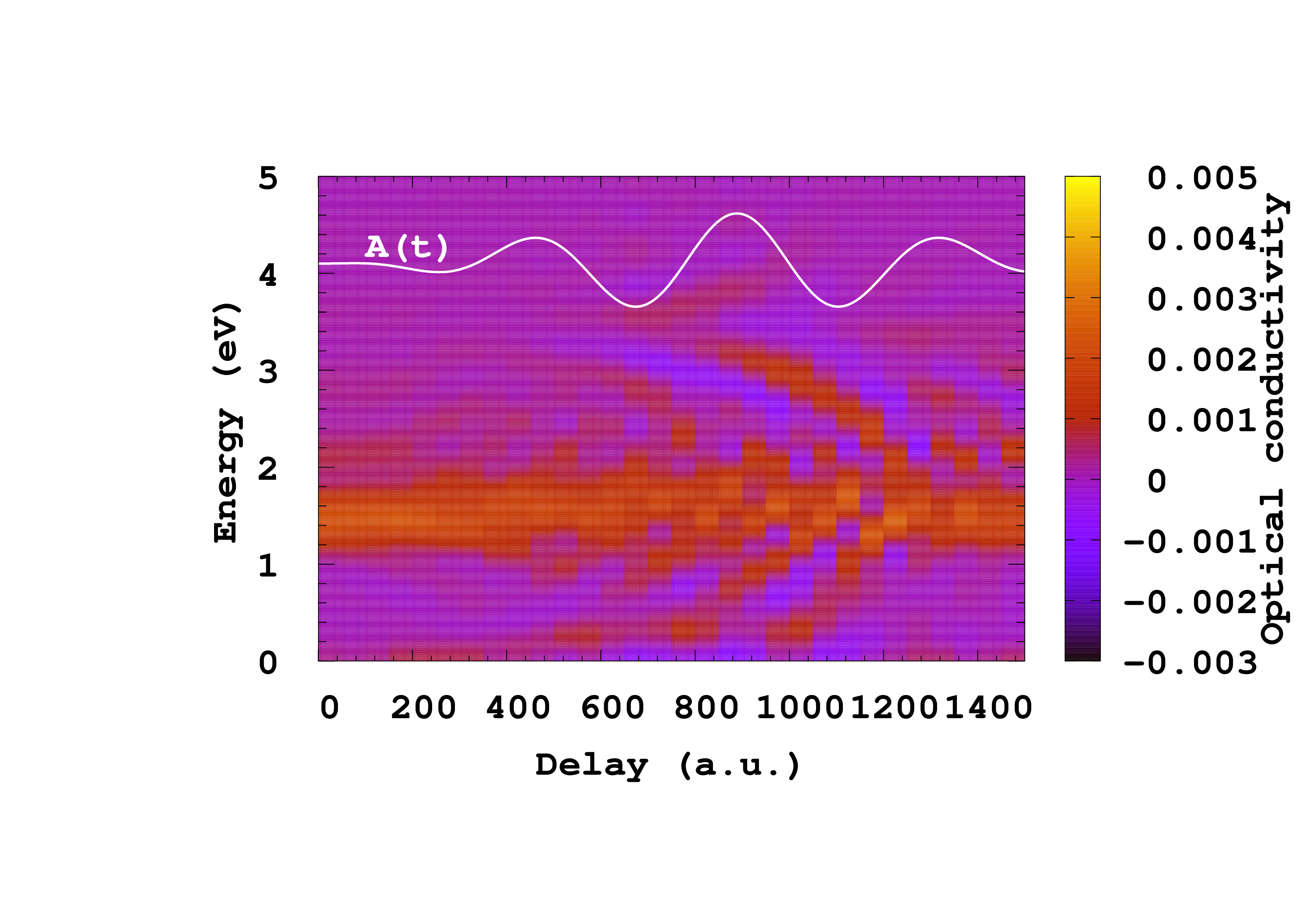
In this plot, we show how the conductivity changes versus time. We could equally plot the change in conductivity (by subtracting the conductivity at equilibrium, i.e., for zero delay) or compute the change in dielectric function, optical absorption, or reflectivity. These different options are all easily obtained once the conductivity is computed.