Kronig-Penney Model

The Kronig-Penney model is a 1D system that demonstrates band gaps, which relate to the allowed energies for electrons in a material. In this tutorial we calculate the bandstructure for Kronig-Penney Model. The Kronig-Penney Model has a periodic potential of

\[ V(x) = \begin{cases} V_0 & -b < x < 0 \cr 0 & 0 < x < a \end{cases} \]

Where b is the width of each barrier, and a is the spacing between them.

!mkdir 7-Kronig-Penney-Model

Input

The following input file will be used for the ground state calculation:

%%writefile 7-Kronig-Penney-Model/inp

stdout = 'stdout_gs.txt'
stderr = 'stderr_gs.txt'

CalculationMode = gs
ExtraStates = 4
PeriodicDimensions = 1
Dimensions = 1
TheoryLevel = independent_particles

a = 5
b = 1
V = 3

Lsize = (a + b)/2

%LatticeParameters
  a + b
%

Spacing = .0075

%Species
 "A" | species_user_defined | potential_formula | "(x>-b)*V*(x<0)" | valence | 1
%

%Coordinates
 "A" | 0 |
%

%KPointsGrid
 11 |
%

%KPointsPath
  11 |
 0.0 |
 0.5 |
%

ConvEigenError = true

%Output
 potential
 wfs
%
OutputFormat = axis_x
OutputWfsNumber = "1,2"

Writing 7-Kronig-Penney-Model/inp

!cd 7-Kronig-Penney-Model && octopus

from postopus import Run
import matplotlib.pyplot as plt

run = Run("7-Kronig-Penney-Model")
wf = run.scf.wf().isel(step=-1).real
v0 = run.scf.v0().isel(step=-1)

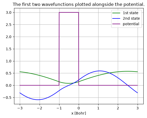
fig, ax = plt.subplots()

wf.sel(st=1, k=1).plot(ax=ax, label="1st state", color="green")
wf.sel(st=2, k=1).plot(ax=ax, label="2nd state", color="blue")
v0.plot(ax=ax, label="potential", color="purple")

ax.set_title("The first two wavefunctions plotted alongside the potential.")
ax.set_ylabel("")
ax.grid(True)
ax.legend();

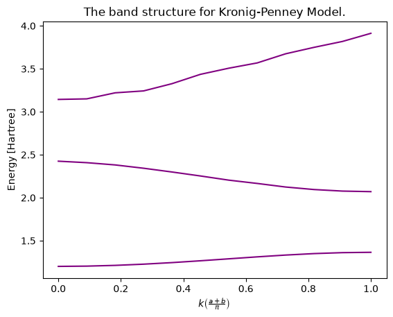
Bandstructure

To calculate the bandstructure simply change the CalculationMode to unocc.

%%writefile 7-Kronig-Penney-Model/inp

stdout = 'stdout_unocc.txt'
stderr = 'stderr_unocc.txt'

CalculationMode = unocc
ExtraStates = 4
PeriodicDimensions = 1
Dimensions = 1
TheoryLevel = independent_particles

a = 5
b = 1
V = 3

Lsize = (a + b)/2

%LatticeParameters
 a + b
%

Spacing = .0075

%Species
 "A" | species_user_defined | potential_formula | "(x>-b)*V*(x<0)" | valence | 1
%

%Coordinates
 "A" | 0 |
%

%KPointsGrid
 11 |
%

%KPointsPath
 11 |
 0.0 |
 0.5 |
%

ConvEigenError = true

Overwriting 7-Kronig-Penney-Model/inp

!cd 7-Kronig-Penney-Model && octopus

To plot the bandstructure, we will use postopus.

run = Run("7-Kronig-Penney-Model")
run.scf.bandstructure()[["band_3", "band_4", "band_5"]].plot(
    color="purple", legend=False
)
plt.xlabel(r"$k \left(\frac{a+b}{\pi}\right)$")
plt.ylabel("Energy [Hartree]")
plt.title("The band structure for Kronig-Penney Model.");

References

1. Sidebottom DL. Fundamentals of condensed matter and crystalline physics: an introduction for students of physics and materials science. New York: Cambridge University Press; 2012.

Tutorial Validation Checks

import numpy as np

ev = run.scf.eigenvalues()

ev is a pandas Dataframe with the following indeces and columns:

ev.index

MultiIndex([( 1, 1),
            ( 1, 2),
            ( 1, 3),
            ( 1, 4),
            ( 1, 5),
            ( 2, 1),
            ( 2, 2),
            ( 2, 3),
            ( 2, 4),
            ( 2, 5),
            ...
            (22, 1),
            (22, 2),
            (22, 3),
            (22, 4),
            (22, 5),
            (23, 1),
            (23, 2),
            (23, 3),
            (23, 4),
            (23, 5)],
           names=['k', 'st'], length=115)

ev.columns

Index(['Spin', 'Eigenvalue', 'Occupation', 'Error'], dtype='str')

We can extract the eigenvalues for k-point i, by ev.Eigenvalue.loc[i].

np.testing.assert_allclose(ev.Eigenvalue.loc[1].to_numpy(), 
                           [0.137751, 0.60848 , 1.200825, 2.426264, 3.127127], rtol=0.001)

np.testing.assert_allclose(ev.Eigenvalue.loc[2].to_numpy(),
                           [0.138834, 0.602898, 1.212622, 2.380146, 3.199639], rtol=0.001)

np.testing.assert_allclose(ev.Eigenvalue.loc[5].to_numpy(),
                           [0.141801, 0.588478, 1.244819, 2.297815, 3.348898], rtol=0.001)

np.testing.assert_allclose(ev.Eigenvalue.loc[10].to_numpy(),
                           [0.152085, 0.545918, 1.360813, 2.076682, 3.841202], rtol=0.001)

np.testing.assert_allclose(ev.Eigenvalue.loc[15].to_numpy(),
                           [0.140121, 0.596494, 1.226601, 2.342423, 3.242761], rtol=0.001)

np.testing.assert_allclose(ev.Eigenvalue.loc[20].to_numpy(),
                           [0.149705, 0.554934, 1.332629, 2.12374, 3.674789], rtol=0.001)