Optical Spectra Of Solids

In this tutorial we will explore how to compute the optical properties of bulk systems from real-time TDDFT using Octopus. Two methods will be presented, one for computing the optical conductivity from the electronic current and another one computing directly the dielectric function using the so-called “gauge-field” kick method. Note that some of the calculations in this tutorial are quite heavy computationally, so they might require to run in parallel over a several cores to finish in a reasonable amount of time.

import matplotlib.pyplot as plt
import numpy as np
import pandas as pd
from postopus import Run
import psutil

!mkdir -p 3-optical-spectra-of-solids/optical-conductivity

cpu_count = min(psutil.cpu_count(logical=False), 8)

Number of cores in this tutorial:

cpu_count

8

Groundstate

Input

As always, we will start with the input file for the ground state, here of bulk silicon. In this case we will use a primitive cell of Si, composed of two atoms, as used in the Getting started with periodic systems tutorial:

%%writefile 3-optical-spectra-of-solids/optical-conductivity/inp

stdout = 'stdout_gs.txt'
stderr = 'stderr_gs.txt'

CalculationMode = gs

PeriodicDimensions = 3

Spacing = 0.5

%LatticeVectors
 0.0 | 0.5 | 0.5
 0.5 | 0.0 | 0.5
 0.5 | 0.5 | 0.0
%

a = 10.18
%LatticeParameters
 a | a | a
%

%ReducedCoordinates
 "Si" | 0.0 | 0.0 | 0.0
 "Si" | 1/4 | 1/4 | 1/4
%

nk = 2
%KPointsGrid
 nk  | nk  | nk
 0.5 | 0.5 | 0.5
 0.5 | 0.0 | 0.0
 0.0 | 0.5 | 0.0
 0.0 | 0.0 | 0.5
%
KPointsUseSymmetries = yes
%SymmetryBreakDir
 1 | 0 | 0
%

Eigensolver = chebyshev_filter
ExtraStates = 4

Writing 3-optical-spectra-of-solids/optical-conductivity/inp

The description of most variables is given in the Getting started with periodic systems. Here we only added one variable:

• SymmetryBreakDir: this input variable is used here to specify that we want to remove from the list of possible symmetries to be used the ones that are broken by a perturbation along the x axis. Indeed, we will later apply a perturbation along this direction, which will break the symmetries of the system.

Output

Now run Octopus using the above input file.

!cd 3-optical-spectra-of-solids/optical-conductivity && octopus

The important thing to note from the output is the effect of the SymmetryBreakDir input option:

***************************** Symmetries *****************************
Space group No.  227
International: Fd-3m
Schoenflies: Oh^7
Info: The system has     4 symmorphic symmetries that can be used.
  Index                Rotation matrix                      Fractional translations
    1 :     1   0   0     0   1   0     0   0   1      0.000000    0.000000    0.000000
    2 :    -1   0   0    -1   0   1    -1   1   0      0.000000    0.000000    0.000000
    3 :    -1   0   0    -1   1   0    -1   0   1      0.000000    0.000000    0.000000
    4 :     1   0   0     0   0   1     0   1   0      0.000000    0.000000    0.000000
Info: The system also has     0 nonsymmorphic symmetries (not used for electrons).
**********************************************************************

Here Octopus tells us that only 4 symmetries can be used, whereas without SymmetryBreakDir, 24 symmetries could have been used. Since only some symmetries are used, twelve ‘‘k’’-points are generated, instead of two ‘‘k’’-points if we would have used the full list of symmetries. If we had not used symmetries at all, we would have 32 ‘‘k’’-points instead.

Optical conductivity

We now turn our attention to the calculation of the optical conductivity. For this, we will apply to our system a time-dependent vector potential perturbation in the form of a Heaviside step function. This corresponds to applying a delta-kick electric field. However, because electric fields (length gauge) are not compatible with the periodicity of the system, we work here with vector potentials (velocity gauge).

The corresponding input file is given below.

%%writefile 3-optical-spectra-of-solids/optical-conductivity/inp

stdout = 'stdout_td.txt'
stderr = 'stderr_td.txt'

CalculationMode = td
FromScratch = yes
PeriodicDimensions = 3

Spacing = 0.5

%LatticeVectors
  0.0 | 0.5 | 0.5
  0.5 | 0.0 | 0.5
  0.5 | 0.5 | 0.0
%

a = 10.18
%LatticeParameters
 a | a | a
%

%ReducedCoordinates
 "Si" | 0.0 | 0.0 | 0.0
 "Si" | 1/4 | 1/4 | 1/4
%

nk = 2
%KPointsGrid
  nk |  nk |  nk
 0.5 | 0.5 | 0.5
 0.5 | 0.0 | 0.0
 0.0 | 0.5 | 0.0
 0.0 | 0.0 | 0.5
%
KPointsUseSymmetries = yes
%SymmetryBreakDir
  1 | 0 | 0
%

ExperimentalFeatures = yes

%TDExternalFields
 vector_potential | 1.0 | 0.0 | 0.0 | 0.0 | "envelope_step"
%

%TDFunctions
 "envelope_step" | tdf_from_expr | "0.01*step(t)"
%

%TDOutput
 total_current
%

TDTimeStep = 0.3
TDPropagationTime = 1500
TDExponentialMethod = lanczos

Overwriting 3-optical-spectra-of-solids/optical-conductivity/inp

Most variables have already been discussed in the different prior tutorials. Here are the most important considerations:

• TDOutput: We ask for outputting the total electronic current. Without this, we will not be able to compute the optical conductivity.

• TDExternalFields: We applied a vector potential perturbation along the ‘‘x’’ axis using.

• TDFunctions: We defined a step function, an used a strength of the perturbation of 0.01. Note that the strength of the perturbation should be small enough, to guaranty that we remain in the linear response regime. Otherwise, nonlinear effects are coupling different frequencies and a an approach based of the “kick” method is not valid anymore. Note that if you would have forgotten above to specify SymmetryBreakDir, the code could would have stopped and let you know that your laser field is breaking some of the symmetries of the system:

******************************* FATAL ERROR *******************************
  \*\* Fatal Error (description follows)
  \* In namespace Lasers:
  \*--------------------------------------------------------------------
  \* The lasers break (at least) one of the symmetries used to reduce the k-points  .
  \* Set SymmetryBreakDir accordingly to your laser fields.
***********************************************************************

Now run Octopus using the above input file.

!cd 3-optical-spectra-of-solids/optical-conductivity && mpirun -n $cpu_count octopus

After the calculation is finished, you can find in the td.general folder the total_current file, that contains the computed electronic current. From it, we want to compute the optical conductivity. This is done by running the utility oct-conductivity . Before doing so, we need to specify the type of broadening that we want to apply to our optical spectrum. In real time, this correspond to applying a damping function to the time signal. For instance, the Lorentzian broadening that we will employ in this tutorial is given by an exponential damping. To specify it, simply add the line

PropagationSpectrumDampMode = exponential

to your input file before running the oct-conductivity utility. Running the utility produces the file td.general/conductivity , which contains the optical conductivity σ(ω) of our system. However, note that at the moment the obtained conductivity is not scaled properly, it is normalized to the volume and proportional to the strength of the perturbation. Hence, in order to obtain the absorption spectrum, we need to compute

\(ℑ[ϵ(ω)]= \frac{4\pi V}{E_0\omega} ℜ[σ(ω)]\)

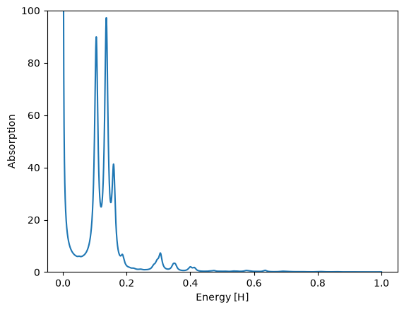
where V is the volume of the system (in this case 10.18^3/4) and E_0 is the strength of the kick (here 0.01). Since our perturbation was along the ‘‘x’’ direction, we want to plot the ‘‘x’’ component of the conductivity. Therefore, in the end, we need to plot the second column of td.general/conductivity multiplied by appropriate factor versus the energy (first column). You can see how the spectrum should look like in Fig. 1. Because we are computing a current-current response, the spectrum exhibits a divergence at low frequencies. This numerical artifact vanishes when more ‘‘k’’-points are included in the simulation.

!echo "PropagationSpectrumDampMode = exponential" >> 3-optical-spectra-of-solids/optical-conductivity/inp

!cd 3-optical-spectra-of-solids/optical-conductivity && oct-conductivity

Looking at the optical spectrum, we observe three main peaks. These correspond to the \(E_0\), \(E_1\), and \(E_1\) critical points of the bandstructure of silicon. Of course, the shape of the spectrum is not converged because we used too few ‘‘k’’-points to sample the Brillouin zone. Remember that you should also perform a convergence study of the spectrum with respect with the relevant parameters. In this case those would be the spacing and the ‘‘k’’-points.

run = Run("3-optical-spectra-of-solids/optical-conductivity")
df = run.td.conductivity()

E0 = 0.01
c = 137

df["absorption"] = 4 * np.pi * c / E0 * df["Conductivity_ReX"] / df["Energy"]
fig, axs = plt.subplots()
df.plot(ax=axs, x="Energy", y="absorption", legend=False, ylim=[0, 100])
axs.set_xlabel("Energy [H]")
axs.set_ylabel("Absorption");

Dielectric function using gauge field kick

Let us now look at a different way to compute the dielectric function of a solid. The dielectric function can be defined from the link between the macroscopic total electric field (or vector potential) and the external electric field. Thus, one can solve the Maxwell equation for computing the macroscopic induced field in order to get the total vector potential acting on the system.

This is the reasoning behind the gauge-field method, as proposed in Ref \(^1\).

Note that before running this input file, we need to redo a GS calculation setting ‘’nk=5’’, to have the same ‘‘k’’-point grid as in the above input file.

!mkdir -p 3-optical-spectra-of-solids/gauge-field-kick

%%writefile 3-optical-spectra-of-solids/gauge-field-kick/inp

stdout = 'stdout_gs.txt'
stderr = 'stderr_gs.txt'

CalculationMode = gs

PeriodicDimensions = 3

Spacing = 0.5

%LatticeVectors
 0.0 | 0.5 | 0.5
 0.5 | 0.0 | 0.5
 0.5 | 0.5 | 0.0
%

a = 10.18
%LatticeParameters
 a | a | a
%

%ReducedCoordinates
 "Si" | 0.0 | 0.0 | 0.0
 "Si" | 1/4 | 1/4 | 1/4
%

nk = 5
%KPointsGrid
 nk  | nk  | nk
 0.5 | 0.5 | 0.5
 0.5 | 0.0 | 0.0
 0.0 | 0.5 | 0.0
 0.0 | 0.0 | 0.5
%
KPointsUseSymmetries = yes
%SymmetryBreakDir
 1 | 0 | 0
%

Eigensolver = chebyshev_filter
ExtraStates = 4

Writing 3-optical-spectra-of-solids/gauge-field-kick/inp

!cd 3-optical-spectra-of-solids/gauge-field-kick && mpirun -n $cpu_count octopus

%%writefile 3-optical-spectra-of-solids/gauge-field-kick/inp

stdout = 'stdout_td.txt'
stderr = 'stderr_td.txt'

CalculationMode = td
FromScratch = yes

PeriodicDimensions = 3

Spacing = 0.5

%LatticeVectors
  0.0 | 0.5 | 0.5
  0.5 | 0.0 | 0.5
  0.5 | 0.5 | 0.0
%

a = 10.18
%LatticeParameters
 a | a | a
%

%ReducedCoordinates
 "Si" | 0.0 | 0.0 | 0.0
 "Si" | 1/4 | 1/4 | 1/4
%

nk = 5
%KPointsGrid
  nk |  nk |  nk
 0.5 | 0.5 | 0.5
 0.5 | 0.0 | 0.0
 0.0 | 0.5 | 0.0
 0.0 | 0.0 | 0.5
%
KPointsUseSymmetries = yes
%SymmetryBreakDir
  1 | 0 | 0
%

%GaugeVectorField
 0.1 | 0 | 0
%

TDTimeStep = 0.2
TDPropagationTime = 1500
TDExponentialMethod = lanczos

Overwriting 3-optical-spectra-of-solids/gauge-field-kick/inp

!cd 3-optical-spectra-of-solids/gauge-field-kick && mpirun -n $cpu_count octopus

Also here, we need to add the option PropagationSpectrumDampMode = exponential to the input file before running the oct-dielectric-function utility.

!echo "PropagationSpectrumDampMode = exponential" >> 3-optical-spectra-of-solids/gauge-field-kick/inp

!cd 3-optical-spectra-of-solids/gauge-field-kick && oct-dielectric-function

Parser warning: possible mistakes in input file.
List of variable assignments not used by parser:
symmetrybreakdir[0][2] = 0.000000
symmetrybreakdir[0][1] = 0.000000
symmetrybreakdir[0][0] = 1.000000
kpointsgrid[4][2] = 0.500000
kpointsgrid[4][1] = 0.000000
kpointsgrid[4][0] = 0.000000
kpointsgrid[3][2] = 0.000000
kpointsgrid[3][1] = 0.500000
kpointsgrid[3][0] = 0.000000
kpointsgrid[2][2] = 0.000000
kpointsgrid[2][1] = 0.000000
kpointsgrid[2][0] = 0.500000
kpointsgrid[1][2] = 0.500000
kpointsgrid[1][1] = 0.500000
kpointsgrid[1][0] = 0.500000
kpointsgrid[0][2] = 5.000000
kpointsgrid[0][1] = 5.000000
kpointsgrid[0][0] = 5.000000
reducedcoordinates[1][3] = 0.250000
reducedcoordinates[1][2] = 0.250000
reducedcoordinates[1][1] = 0.250000
reducedcoordinates[1][0] = "Si"
reducedcoordinates[0][3] = 0.000000
reducedcoordinates[0][2] = 0.000000
reducedcoordinates[0][1] = 0.000000
reducedcoordinates[0][0] = "Si"

Note that before running this input file, you need to redo a GS calculation setting nk = 5, to have the same ‘‘k’’-point grid as in the above input file.

Compared to the previous TD calculation, we have made few changes:

• GaugeVectorField: This activates the calculation of the gauge field and its output. This replaces the laser field used in the previous method.

• KPointsGrid: We used here a much denser ‘‘k’’-point grid. This is needed because of the numerical instability of the gauge-field method for very low number of ‘‘k’’-points.

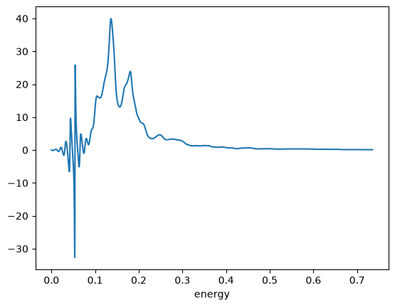
After running this input file with Octopus, we can run the utility oct-dielectric-function , which produces the output td.general/dielectric_function . In this case we are interested in the imaginary part of the dielectric function along the ‘‘x’’ direction, which correspondents to the third column of the file. You can see how the spectra looks like in Fig. 2. As we can see, below the bandgap, we observe some numerical noise. This is again due to the fact that the spectrum is not properly converged with respect to the number of ‘‘k’’-points and vanishes if sufficient ‘‘k’’-points are used. Apart from this, we now obtained a much more converged spectrum, with the main three features starting to resemble the fully-converged spectrum.

run = Run("3-optical-spectra-of-solids/gauge-field-kick")
dielectric_function = run.td.dielectric_function()
dielectric_function["Im"].plot();

References

1. Bertsch, G. F. and Iwata, J.-I. and Rubio, Angel and Yabana, K., Real-space, real-time method for the dielectric function, Phys. Rev. B 62 7998 (2000);

Tutorial Validation Checks

from tutorial_helpers import extract_peak

Optical Conductivity

np.testing.assert_allclose(extract_peak(df["Energy"][1:], df["absorption"][1:], order=1, sort_by="peak_heights"), (0.1361, 0.012461248353899862, 97.3051313590378), rtol=0.01)

np.testing.assert_allclose(extract_peak(df["Energy"][1:], df["absorption"][1:], order=2, sort_by="peak_heights"), (0.1046, 0.0097453047415373, 91.11769745008424), rtol=0.01)

np.testing.assert_allclose(extract_peak(df["Energy"][1:], df["absorption"][1:], order=3, sort_by="peak_heights"), (0.1589, 0.006710551635557921, 41.567446701075234), rtol=0.01)

Gauge field kick

np.testing.assert_allclose(extract_peak(dielectric_function.index.to_numpy(), dielectric_function["Im"].to_numpy(), sort_by="peak_heights", order=1), (0.13634, 0.027171867649568582, 39.995), rtol=0.01)

np.testing.assert_allclose(extract_peak(dielectric_function.index.to_numpy(), dielectric_function["Im"].to_numpy(), sort_by="peak_heights", order=2), (0.054389, 0.0020713424403924832, 25.9776), rtol=0.01)

np.testing.assert_allclose(extract_peak(dielectric_function.index.to_numpy(), dielectric_function["Im"].to_numpy(), sort_by="peak_heights", order=3), (0.180439, 0.019163074898570942, 23.9243), rtol=0.01)