Visualization
In this tutorial we will explain how to visualize outputs from Octopus. Several different file formats are available in Octopus that are suitable for a variety of visualization software. We will not cover all of them here. See Visualization for more information.
mkdir -p 4-visualization
Benzene molecule
As an example, we will use the benzene molecule. At this point, the input should be quite familiar to you:
%%writefile 4-visualization/inp

stdout = "stdout_gs.txt"
stderr = "stderr_gs.txt"

CalculationMode = gs
UnitsOutput = eV_Angstrom

Eigensolver = chebyshev_filter
ExtraStates = 4

Radius = 5*angstrom
Spacing = 0.15*angstrom

%Output
  density | netcdf
%

XYZCoordinates = "benzene.xyz"
Writing 4-visualization/inp
Coordinates are in this case given in the benzene.xyz file. This file should look like:
%%writefile 4-visualization/benzene.xyz
12
   Geometry of benzene (in Angstrom)
   C  0.000  1.396  0.000
   C  1.209  0.698  0.000
   C  1.209 -0.698  0.000
   C  0.000 -1.396  0.000
   C -1.209 -0.698  0.000
   C -1.209  0.698  0.000
   H  0.000  2.479  0.000
   H  2.147  1.240  0.000
   H  2.147 -1.240  0.000
   H  0.000 -2.479  0.000
   H -2.147 -1.240  0.000
   H -2.147  1.240  0.000
Writing 4-visualization/benzene.xyz
Here we have used the new input variable Output. This tells Octopus what quantities to output in which format.
In this case we ask Octopus to output the density in the netcdf format, which saves the full 3D data in binary format and can efficiently be used with postopus. Other visualization tools may need specific other output formats, as mentioned below. For performance and disk consumption reasons you should only keep the option that corresponds to the program you will use and the quantities that you will analyse. Take a look at the documentation on variables Output and OutputFormat for the full list of possible quantities to output and formats to visualize them in.
!cd 4-visualization && octopus
Visualization
Post-processing of the data generated by Octopus can be done in many different ways. Here we will introduce some of the most common tools including Postopus which is a python tool developed primarily for the POST-processing of octOPUS data.
Postopus
Postopus can be installed using pip install "postopus[recommended]" on a command line.
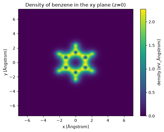
A sample program to plot a slice density of benzene in the xy plane (z=0) is shown below:
from postopus import Run
import matplotlib.pyplot as plt

run = Run("./4-visualization") # Collect the output files of the octopus run be creating a Run object
density = run.scf.density() # Load the data from files `density.ncdf`
converged = density[-1]  # Get the density of the last (converged) iteration
density_z0 = converged.sel(z=0, method="nearest")  # Select the xy plane (nearest data point to z=0)

# Plot the selected data
density_z0.plot(x="x", y="y")
plt.title("Density of benzene in the xy plane (z=0)");
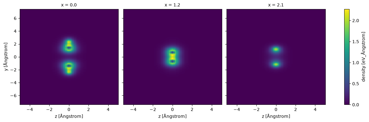
We can also plot multiple slice along the x-axis:
xa = converged.sel(x=[0, 1.209, 2.147], method="nearest")
xa.plot(col="x", figsize=(13,4), aspect="equal");
Postopus provides various tools for exploring the data, using holoviews is well suited for interactive work:
import holoviews as hv
from holoviews import opts  # For setting defaults

hv.extension("bokeh")  # Allow for interactive plots

# Choose color scheme similar to matplotlib
opts.defaults(
    opts.Image(cmap="viridis", width=500, height=400),
)

# Holoviews
ds = hv.Dataset(converged).to(hv.Image, kdims=["x", "y"]).opts(
    colorbar=True, clim=(0, converged.values.max())
)
ds.dimensions()[0].default = converged.z.values[len(converged.z) // 2] # Set inital position of the z-slider to the middle of the molecule
ds


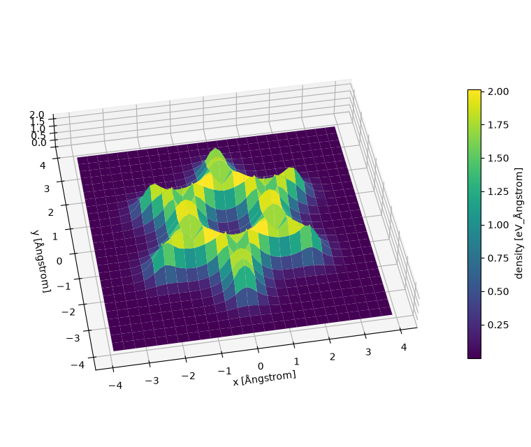
The same data can also be visualised in a 3D plot:
import numpy as np

# Shrink x/y coordinates a little
data = density_z0.sel(x=slice(-4,4), y=slice(-4,4))

fig, ax = plt.subplots(subplot_kw={"projection": "3d"}, figsize=(10, 10))
X, Y = np.meshgrid(data.coords["x"], data.coords["y"], indexing="ij")
Z = data.values

surf = ax.plot_surface(X, Y, Z, cmap="viridis")
ax.set_box_aspect(aspect = (1,1,0.15))
ax.view_init(elev=45, azim=-100)
ax.set_xlabel("x [Ångstrom]")
ax.set_ylabel("y [Ångstrom]")
fig.colorbar(surf, shrink=0.5, label="density [eV_Ångstrom]");
More information about postopus can be found in the postopus documentation. This example is covered in more detail here and a quick start for postopus is available here.
Gnuplot
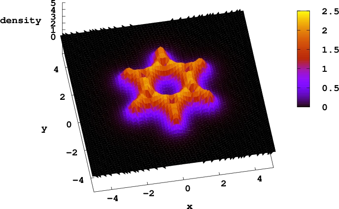
Electronic density of benzene along the z=0 plane. Generated in Gnuplot with the ‘pm3d’ option.
Visualization of the fields in 3-dimensions is complicated. In many cases it is more useful to plot part of the data, for example the values of a scalar field along a line of plane that can be displayed as a 1D or 2D plot.
The gnuplot program is very useful for making these types of plots (and many more) and can directly read Octopus output. For the following two examples you would need to specify axis_x and plane_z in the Output block. First type gnuplot to enter the program’s command line. Now to plot a the density along a line (the X axis in this case) type
plot "static/density.y=0,z=0" w l
To plot a 2D field, for example the density in the plane z=0, you can use the command
splot "static/density.z=0" w l
If you want to get a color scale for the values of the field use w pm3d instead of w l.
Gnuplot script
set xlabel "x"
set ylabel "y"
set zlabel "density"
set t postscript enhanced color font “Monospace-Bold,20” landscape size 11,8.5
set output “benzene_2D.eps”
set key left
set rmargin 4.5
set lmargin 9.5
set tmargin 3.2
set bmargin 5.5
set view 20, 350
splot [-5:5][-5:5][0:5] “static/density.z=0” w pm3d t ‘’
VisIt
The program VisIt is an open-source data visualizer developed by Lawrence Livermore National Laborartory. It supports multiple platforms including Linux, OS X and Windows, most likely you can download a precompiled version for your platform here.
For this tutorial you need to have Visit installed and running. VisIt can read several formats, the most convenient for Octopus data is the cube format: OutputFormat = cube. This is a common format that can be read by several visualization and analysis programs, it has the advantage that includes both the requested scalar field and the geometry in the same file. Visit can also read other formats that Octopus can generate like xyz, XSF (partial support), and VTK.
The following video contains the instruction on how to open a cube file in VisIt. Note that the video has subtitles in case you don’t have audio in your current location, you can enable them by clicking the “CC” button.
XCrySDen
Atomic coordinates (finite or periodic), forces, and functions on a grid can be plotted with the free program XCrysDen. Its XSF format also can be read by V_Sim and VESTA. Beware, these all probably assume that your output is in Angstrom units (according to the specification), so use UnitsOutput = eV_Angstrom, or your data will be misinterpreted by the visualization software.
UCSF Chimera
To visualize with UCSF Chimera set OutputFormat = dx.
Once having UCSF Chimera installed and opened, open the benzene.xyz file from “File > Open”.
To open the .dx file, go to “Tools > Volume Data > Volume Viewer”. A new window opens. There go to “File > Open” and select static/density.dx.
To “color” the density go to “Tools > Surface Color”. A new dialog opens and there choose “Browse” to open the vh.dx file. Then click “Color” and you should have an image similar to the below one.
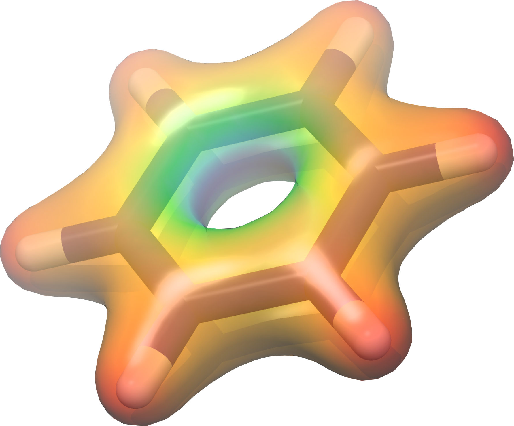
Ground-state density plotted with UCSF Chimera for the benzene molecule, colored according to the value of the electrostatic potential
Tutorial Validation Checks
from postopus import Run
import numpy as np

run = Run("4-visualization")
total_energy = run.scf.info.get_total_energy()
assert(run.scf.info.scf_is_converged())
np.testing.assert_allclose(float(total_energy), -1026.736189, atol=1e-4)