Total energy convergence
In this tutorial we will show how to converge a quantity of interest (the total energy) with respect to the parameters that define the real-space grid. For this we will use two examples, the Nitrogen atom from the Basic input options tutorial, and a methane molecule.
from pathlib import Path
import pandas as pd
import numpy as np
from postopus import Run
import subprocess
Nitrogen atom: finding a good spacing
The key parameter of a real-space calculation is the spacing between the points of the mesh. The default option in Octopus is to use a Cartesian grid. This is a regular grid where the spacing along each Cartesian direction is the same. The first step in any calculation should then be making sure that this spacing is good enough for our purposes. This should be done through a convergence study, very similar to the ones performed in plane-wave calculations.
The needed spacing essentially depends on the pseudopotentials that are being used. The idea is to repeat a series of ground-state calculations, with identical input files except for the grid spacing. There are many different ways of doing it, the simplest one being to change the input file by hand and run Octopus each time. Another option is to use a little python script like the one below.
As a first example, we will use the Nitrogen atom from the previous tutorial.
mkdir -p 3-total_energy_convergence/1-spacing_nitrogen
Create runs for different spacings
In order to change the value of the spacing for each calculation, we define the content of the inp file as a string containing a placeholder {spacing_value}.
inp_template_Nitrogen = """
CalculationMode = gs
UnitsOutput = eV_Angstrom

Eigensolver = chebyshev_filter
ExtraStates = 4

stdout = 'stdout_td_{spacing_value}.txt'
stderr = 'stderr_td_{spacing_value}.txt'

Nitrogen_mass = 14.0

%Species
'N' | species_pseudo | set | standard | lmax | 1 | lloc | 0 | mass | Nitrogen_mass
%

%Coordinates
  'N' | 0 | 0 | 0
%

%Occupations
2 | 1 | 1 | 1
%

BoxShape = sphere
Radius = 5.0*angstrom
Spacing = {spacing_value}*angstrom
"""
We can now loop over a list of spacings (0.26, 0.24, …, 0.14), write an inp file with the desired spacing using our template string and str.format, and run Octopus for that spacing. A separate directory is created for each spacing.
list_of_spacing = [0.26, 0.24, 0.22, 0.20, 0.18, 0.16, 0.14]

for spacing in list_of_spacing:
    print(f"Running octopus for spacing: {spacing}")
    runpath = Path(f"3-total_energy_convergence/1-spacing_nitrogen/run_{spacing}")
    runpath.mkdir(exist_ok=True)
    (runpath / "inp").write_text(inp_template_Nitrogen.format(spacing_value=spacing))
    subprocess.run("octopus", cwd=runpath)
Running octopus for spacing: 0.26
Running octopus for spacing: 0.24
Running octopus for spacing: 0.22
Running octopus for spacing: 0.2
Running octopus for spacing: 0.18
Running octopus for spacing: 0.16
Running octopus for spacing: 0.14
Retrieve and combine data for different spacings
For each spacing we want to extract the total energy as well as the eigenvalues from the info file. Wo do this by using Postopus, a python tool for the post processing of Octopus data.
def get_scf_info(run_path: str):
    """
    Extract Total energy , seigen, peigen from info.
    """
    info = Run(run_path).scf.info

    total_energy = info.get_total_energy()

    eigenvalues = info.get_eigenvalues()
    s_eigen = eigenvalues.loc[1]["Eigenvalue"]
    p_eigen = eigenvalues.loc[2]["Eigenvalue"]

    return {"Total_Energy": total_energy, "S_eigen": s_eigen, "P_eigen": p_eigen}
records = []
for spacing in list_of_spacing:
    records.append(get_scf_info(f"3-total_energy_convergence/1-spacing_nitrogen/run_{spacing}"))

df = pd.DataFrame.from_records(records, index=list_of_spacing)
df.index.name = "Spacing"
df
| Total_Energy | S_eigen | P_eigen | |
|---|---|---|---|
| Spacing | |||
| 0.26 | -256.568183 | -19.856254 | -6.753300 |
| 0.24 | -260.262411 | -18.816300 | -7.085016 |
| 0.22 | -262.607263 | -18.190682 | -7.321587 |
| 0.20 | -262.935468 | -18.096063 | -7.363765 |
| 0.18 | -262.241139 | -18.282857 | -7.302310 |
| 0.16 | -261.800624 | -18.390803 | -7.251495 |
| 0.14 | -261.819578 | -18.386175 | -7.256964 |
# to normalise the plot, shift values such that everything is 0 at spacing 0.14
df_normalised = df - df.iloc[-1]

# plot total energy, S-eigen, P-eigen trend against Spacing
df_normalised.plot(
    style="o-",
    grid=True,
    title="Convergence with spacing of N",
    ylabel="Error (eV)",
    xlabel="Spacing (Å)",
);
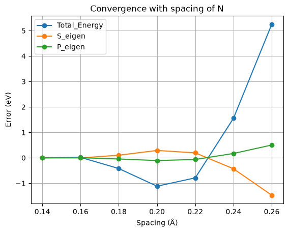
The results, for this particular example, are shown in the figure. In this figure we are actually plotting the error with respect to the most accurate results (smallest spacing). That means that we are plotting the ‘’’difference’’’ between the values for a given spacing and the values for a spacing of 0.14 Å. So, in reading it, note that the most accurate results are at the left (smallest spacing). A rather good spacing for this nitrogen pseudopotential seems to be 0.18 Å. However, as we are usually not interested in total energies, but in energy differences, probably a larger one may also be used without compromising the results.
Methane molecule
We will now move on to a slightly more complex system, the methane molecule CH4, and add a convergence study with respect to the box size.
Input
As usual, the first thing to do is create an input file for this system. From our basic chemistry class we know that methane has a tetrahedral structure. The only other thing required to define the geometry is the bond length between the carbon and the hydrogen atoms. If we put the carbon atom at the origin, the hydrogen atoms have the coordinates given in the following input file:
inp_template_methane = """
stdout = 'stdout_gs.txt'
stderr = 'stderr_gs.txt'

CalculationMode = gs
UnitsOutput = eV_Angstrom

Eigensolver = chebyshev_filter
ExtraStates = 4

Radius = {radius_value}*angstrom
Spacing = {spacing_value}*angstrom

CH = 1.2*angstrom
%Coordinates
 "C" |           0 |          0 |           0
 "H" |  CH/sqrt(3) | CH/sqrt(3) |  CH/sqrt(3)
 "H" | -CH/sqrt(3) |-CH/sqrt(3) |  CH/sqrt(3)
 "H" |  CH/sqrt(3) |-CH/sqrt(3) | -CH/sqrt(3)
 "H" | -CH/sqrt(3) | CH/sqrt(3) | -CH/sqrt(3)
%
"""
Here we define a variable CH that represents the bond length between the carbon and the hydrogen atoms, which simplifies the writing of the coordinates. We start with a bond length of 1.2 Å but that’s not so important at the moment, since we can optimize it later (for more information see the Geometry optimization tutorial). (You should not use 5 Å or so, but something slightly bigger than 1 Å is fine.)
Some notes concerning the input file:
We do not tell Octopus explicitly which BoxShape to use. The default is a union of spheres centered around each atom. This turns out to be the most economical choice in almost all cases.
We also do not specify the %Species block. In this way, Octopus will use default pseudopotentials for both Carbon and Hydrogen. This should be OK in many cases, but, as a rule of thumb, you should do careful testing before using any pseudopotential for serious calculations.
As in the convergence of the spacing above we added the placeholder {radius_value}. Lets first run Octopus in a separate directory for Spacing = 0.22*angstrom and Radius = 3.5*angstrom:
Path(f"3-total_energy_convergence/2-spacing_methane/run_0.22").mkdir(parents=True, exist_ok=True)
Path(f"3-total_energy_convergence/2-spacing_methane/run_0.22/inp").write_text(
    inp_template_methane.format(spacing_value=0.22, radius_value=3.5)
)

subprocess.run(
    "octopus", cwd=f"3-total_energy_convergence/2-spacing_methane/run_0.22"
)
CompletedProcess(args='octopus', returncode=0)
This gives us the following values in the resulting static/info file:
Eigenvalues [eV]
 #st  Spin   Eigenvalue      Occupation
   1   --   -15.990984       2.000000
   2   --    -9.065633       2.000000
   3   --    -9.065633       2.000000
   4   --    -9.065633       2.000000
   5   --     0.267943       0.000000
   6   --     1.933440       0.000000
   7   --     1.933440       0.000000
   8   --     1.933440       0.000000

Energy [eV]:
      Total       =      -219.03759845
      Free        =      -219.03759845
      -----------
      Ion-ion     =       236.08498119
      Eigenvalues =       -86.37576790
      Hartree     =       393.45805964
      Int[n*v_xc] =      -105.38065279
      Exchange    =       -69.66883366
      Correlation =       -11.00057123
      vanderWaals =         0.00000000
      Delta XC    =         0.00000000
      Entropy     =         0.00000000
      -TS         =        -0.00000000
      Photon ex.  =         0.00000000
      Kinetic     =       163.97237638
      External    =      -931.88361077
      Non-local   =       -49.75777859
      Int[n*v_E]  =         0.00000000
Now the question is whether these values are converged or not. This will depend on two things: the BoxShape, as seen above, and the Species. Just like for the Nitrogen atom, the only way to answer this question is to try other values for these variables.
Convergence with the spacing
As before, we will keep all entries in the input file fixed except for the spacing that we will make smaller by 0.02 Å all the way down to 0.1 Å. So you have to run Octopus several times. We use a similar loop as the one from the Nitrogen atom example:
spacing_list = [0.22, 0.20, 0.18, 0.16, 0.14, 0.12, 0.10]

for spacing in spacing_list:
    print(f"Running octopus for spacing: {spacing}")
    runpath = Path(f"3-total_energy_convergence/2-spacing_methane/run_{spacing}")
    runpath.mkdir(exist_ok=True)
    (runpath / "inp").write_text(inp_template_methane.format(spacing_value=spacing, radius_value=3.5))
    subprocess.run("octopus", cwd=runpath)
Running octopus for spacing: 0.22
Running octopus for spacing: 0.2
Running octopus for spacing: 0.18
Running octopus for spacing: 0.16
Running octopus for spacing: 0.14
Running octopus for spacing: 0.12
Running octopus for spacing: 0.1
records = []
for spacing in spacing_list:
    records.append(get_scf_info(f"3-total_energy_convergence/2-spacing_methane/run_{spacing}"))

methane_df = pd.DataFrame.from_records(records, index=spacing_list)
methane_df.index.name = "Spacing"
methane_df
| Total_Energy | S_eigen | P_eigen | |
|---|---|---|---|
| Spacing | |||
| 0.22 | -219.037598 | -15.990982 | -9.065632 |
| 0.20 | -218.584087 | -16.062279 | -9.054185 |
| 0.18 | -218.279511 | -16.136386 | -9.050456 |
| 0.16 | -218.199971 | -16.142663 | -9.046144 |
| 0.14 | -218.179071 | -16.142071 | -9.044088 |
| 0.12 | -218.159816 | -16.145164 | -9.044012 |
| 0.10 | -218.139297 | -16.144259 | -9.042185 |
methane_df.Total_Energy.plot(
    style="o-",
    grid=True,
    title="Convergence with spacing of methane",
    ylabel="Total Energy (eV)",
    xlabel="Spacing (Å)",
);
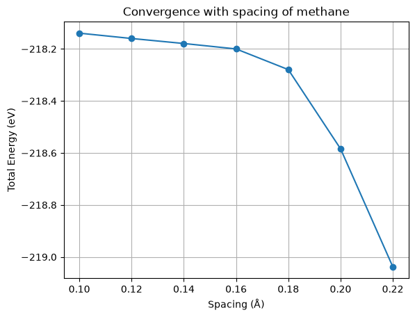
As you can see from this picture, the total energy is converged to within 0.1 eV for a spacing of 0.18 Å. So we will use this spacing for the next calculations.
Convergence with the radius
Now we will see how the total energy changes with the Radius of the box. We will change the radius in steps of 0.5 Å.
radius_list = [2.5, 3.0, 3.5, 4.0, 4.5, 5.0]

for radius in radius_list:
    print(f"Running octopus for radius: {radius}")
    runpath = Path(f"3-total_energy_convergence/3-radius_methane/run_{radius}")
    runpath.mkdir(parents=True, exist_ok=True)
    (runpath / "inp").write_text(inp_template_methane.format(spacing_value=0.18, radius_value=radius))
    subprocess.run("octopus", cwd=runpath)
Running octopus for radius: 2.5
Running octopus for radius: 3.0
Running octopus for radius: 3.5
Running octopus for radius: 4.0
Running octopus for radius: 4.5
Running octopus for radius: 5.0
records = []
for radius in radius_list:
    records.append(get_scf_info(f"3-total_energy_convergence/3-radius_methane/run_{radius}"))

methane_radius_df = pd.DataFrame.from_records(records, index=radius_list)
methane_radius_df.index.name = "Radius"
methane_radius_df
| Total_Energy | S_eigen | P_eigen | |
|---|---|---|---|
| Radius | |||
| 2.5 | -218.071165 | -15.902596 | -8.809031 |
| 3.0 | -218.245630 | -16.085999 | -8.998997 |
| 3.5 | -218.279511 | -16.136386 | -9.050456 |
| 4.0 | -218.286204 | -16.149597 | -9.063791 |
| 4.5 | -218.287589 | -16.153054 | -9.067248 |
| 5.0 | -218.287867 | -16.153894 | -9.068082 |
methane_radius_df.Total_Energy.plot(
    style="o-",
    grid=True,
    title="Convergence with radius of methane",
    ylabel="Total Energy (eV)",
    xlabel="Radius (Å)",
);
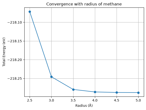
If we again ask for a convergence up to 0.1 eV we should use a radius of 3.5 Å. How does this compare to the size of the molecule? Can you explain why the energy increases (becomes less negative) when one decreases the size of the box?
Tutorial Validation Checks
from postopus import Run
import numpy as np
run = Run("3-total_energy_convergence/2-spacing_methane/run_0.22")
total_energy = run.scf.info.get_total_energy()
evals = run.scf.info.get_eigenvalues()
assert(run.scf.info.scf_is_converged())
np.testing.assert_allclose(float(evals.Eigenvalue[1]), -15.990978, atol=1e-4)
np.testing.assert_allclose(float(evals.Eigenvalue[2]), -9.065537, atol=1e-4)
np.testing.assert_allclose(float(evals.Eigenvalue[3]), -9.065537, atol=1e-4)
np.testing.assert_allclose(float(evals.Eigenvalue[4]), -9.065537, atol=1e-4)
np.testing.assert_allclose(total_energy, -219.03759, atol=1e-4)