Centering a geometry
Before running an Octopus calculation of a molecule, it is always a good idea to run the oct-center-geom utility, which will translate the center of mass to the origin, and align the molecule, by default so its main axis is along the ‘’x’’-axis. Doing this is often helpful for visualization purposes, and making clear the symmetry of the system, and also it will help to construct the simulation box efficiently in the code. The current implementation in Octopus constructs a parallelepiped containing the simulation box and the origin, and it will be much larger than necessary if the system is not centered and aligned. For periodic systems, these considerations are not relevant (at least in the periodic directions).
import matplotlib.pyplot as plt
from postopus import Run
mkdir -p 5-centering
Input
For this example we need two files.
inp
We need only a very simple input file, specifying the coordinates file.
%%writefile 5-centering/inp
XYZCoordinates = "tAB.xyz"

stdout = "stdout.txt"
stderr = "stderr.txt"
Writing 5-centering/inp
tAB.xyz
We will use this coordinates file, for the molecule “trans”-azobenzene, which has the interesting property of being able to switch between “trans” and “cis” isomers by absorption of light.
%%writefile 5-centering/tAB.xyz
24

C   -0.520939   -1.29036    -2.47763
C   -0.580306    0.055376   -2.10547
C    0.530312    0.670804   -1.51903
C    1.71302    -0.064392   -1.30151
C    1.76264    -1.41322    -1.67813
C    0.649275   -2.02387    -2.26419
H   -1.38157    -1.76465    -2.93131
H   -1.48735     0.622185   -2.27142
H    2.66553    -1.98883    -1.51628
H    0.693958   -3.06606    -2.55287
H    0.467127    1.71395    -1.23683
N    2.85908     0.52877    -0.708609
N    2.86708     1.72545    -0.355435
C    4.01307     2.3187      0.237467
C    3.96326     3.66755     0.614027
C    5.0765      4.27839     1.20009
C    6.2468      3.54504     1.41361
C    6.30637     2.19928     1.04153
C    5.19586     1.58368     0.455065
H    5.25919     0.540517    0.17292
H    3.06029     4.24301     0.4521
H    5.03165     5.32058     1.48872
H    7.10734     4.01949     1.86731
H    7.21349     1.63261     1.20754
Writing 5-centering/tAB.xyz
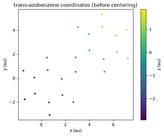
We can use Postopus to plot the initial atom positions:
tAB_xyz = Run("5-centering").geometry.tAB()
# scatter plot xyz coordinates with z as color
fig = plt.figure()
ax = fig.add_subplot(111)
plot = ax.scatter(tAB_xyz["x"], tAB_xyz["y"], c=tAB_xyz["z"], cmap="viridis", s=10)
fig.colorbar(plot).set_label("z (au)")
ax.set_aspect("equal")
plt.title("trans-azobenzene coordinates (before centering)")
ax.set_xlabel("x (au)")
ax.set_ylabel("y (au)");
Centering the geometry
oct-center-geom is a serial utility, and cen be found in the bin directory after installation of Octopus.
When you run the utility, you should obtain a new coordinates file adjusted.xyz for use in your calculations with Octopus.
!cd 5-centering && oct-center-geom
The output is not especially interesting, except for perhaps the symmetries and moment of inertia tensor, which come at the end of the calculation:
***************************** Symmetries *****************************
Symmetry elements : (sigma)
Symmetry group    : Cs
**********************************************************************

Using main axis        1.000000       0.000000       0.000000
Input: [AxisType = inertia]
Center of mass [b] =        5.410288       2.130154      -1.005363
Moment of inertia tensor [amu*b^2]
      6542962.320615     -4064048.884840     -3486905.049193
     -4064048.884840      8371776.892023     -2789525.719087
     -3486905.049193     -2789525.719087     10730451.796958
Isotropic average      8548397.003199
Eigenvalues:            1199576.606657          11623018.898148          12822595.504791
Found primary   axis        0.707107       0.565686       0.424264
Found secondary axis       -0.624695       0.780869      -0.000000
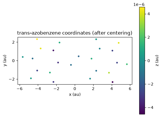
We can use postopus to inspect and plot the adjusted atom positions:
adjusted_xyz = Run("5-centering").geometry.adjusted()
adjusted_xyz
| Atom | x | y | z | |
|---|---|---|---|---|
| 0 | C | -4.585889 | 0.226024 | -1.213000e-06 |
| 1 | C | -3.708710 | 1.313953 | 4.220000e-06 |
| 2 | C | -2.326440 | 1.100724 | -3.973000e-06 |
| 3 | C | -1.813744 | -0.212200 | -3.224000e-06 |
| 4 | C | -2.701456 | -1.296455 | 1.261000e-06 |
| 5 | C | -4.082804 | -1.077778 | -2.714000e-06 |
| 6 | H | -5.655226 | 0.393298 | 3.080000e-07 |
| 7 | H | -4.099857 | 2.323183 | 4.572000e-06 |
| 8 | H | -2.319964 | -2.309962 | -3.023000e-06 |
| 9 | H | -4.763237 | -1.919505 | 4.880000e-07 |
| 10 | H | -1.661299 | 1.954755 | 1.178000e-06 |
| 11 | N | -0.416267 | -0.464957 | -1.203000e-06 |
| 12 | N | 0.416174 | 0.464495 | -1.535000e-06 |
| 13 | C | 1.813651 | 0.211851 | 1.258000e-06 |
| 14 | C | 2.701216 | 1.296242 | -4.440000e-07 |
| 15 | C | 4.082584 | 1.077792 | -2.697000e-06 |
| 16 | C | 4.585854 | -0.225939 | -2.652000e-06 |
| 17 | C | 3.708839 | -1.314014 | 3.466000e-06 |
| 18 | C | 2.326538 | -1.100986 | -1.173000e-06 |
| 19 | H | 1.661513 | -1.955122 | -5.200000e-08 |
| 20 | H | 2.319549 | 2.309681 | 3.720000e-07 |
| 21 | H | 4.762878 | 1.919622 | 4.150000e-06 |
| 22 | H | 5.655226 | -0.393032 | 1.679000e-06 |
| 23 | H | 4.100144 | -2.323183 | -4.572000e-06 |
# scatter plot xyz coordinates from adjusted_df with z as color
fig = plt.figure()
ax = fig.add_subplot(111)
plot = ax.scatter(
    adjusted_xyz["x"], adjusted_xyz["y"], c=adjusted_xyz["z"], cmap="viridis", s=10
)

fig.colorbar(plot).set_label("z (au)")
ax.set_aspect("equal")
plt.title("trans-azobenzene coordinates (after centering)")
ax.set_xlabel("x (au)")
ax.set_ylabel("y (au)");
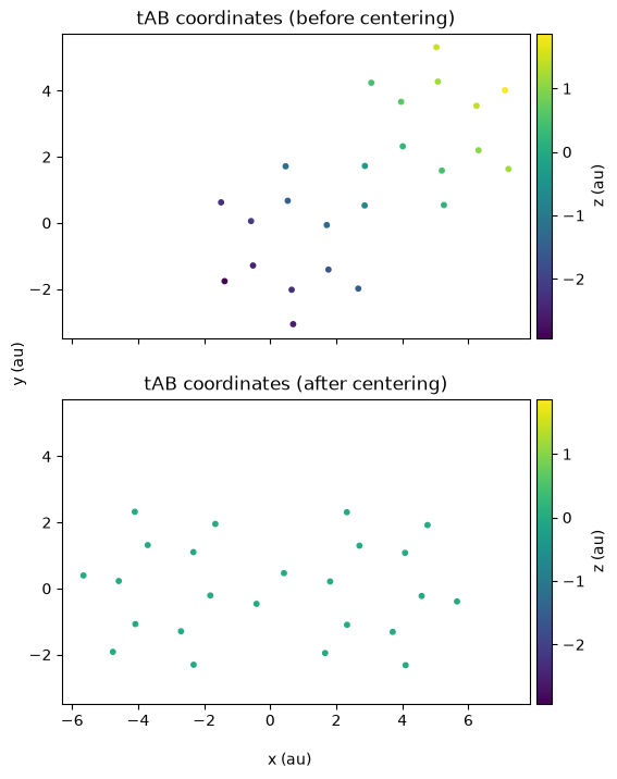
# Plot the two figures one below the other for comparison

fig, (ax1, ax2) = plt.subplots(2, 1, sharex=True, sharey=True, figsize=(8, 8))

z_min = tAB_xyz["z"].min()
z_max = tAB_xyz["z"].max()

sc1 = ax1.scatter(
    tAB_xyz["x"], tAB_xyz["y"], c=tAB_xyz["z"], cmap="viridis", s=10, vmin=z_min, vmax=z_max,
)
ax1.set_aspect("equal")

sc2 = ax2.scatter(
    adjusted_xyz["x"], adjusted_xyz["y"], c=adjusted_xyz["z"], cmap="viridis", s=10, vmin=z_min, vmax=z_max,
)
ax2.set_aspect("equal")

fig.text(0.5, 0.04, "x (au)", ha="center")
fig.text(0.18, 0.5, "y (au)", va="center", rotation="vertical")

cbar1 = plt.colorbar(sc1, ax=ax1, pad=0.01)
cbar1.set_label("z (au)")

cbar2 = plt.colorbar(sc2, ax=ax2, pad=0.01)
cbar2.set_label("z (au)")

ax1.set_title("tAB coordinates (before centering)")
ax2.set_title("tAB coordinates (after centering)");
You can also visualize the coordinates files with xcrysden, Jmol, Avogadro, VMD, Vesta, etc.
You can see more options about how to align the system at AxisType and MainAxis.
Tutorial Validation Checks
from postopus import open_textfile
import numpy as np

run = Run("5-centering")
logfile = open_textfile(run / "stdout.txt")
np.testing.assert_allclose([float(elem) for elem in logfile.grepfield('primary axis')[3:]], [0.707107, 0.565686, 0.424264], atol=1e-4)
np.testing.assert_allclose([float(elem) for elem in logfile.grepfield('secondary axis')[3:]], [-0.624695, 0.780869, 0.0], atol=1e-4)