Triplet excitations

In this tutorial, we will calculate triplet excitations for methane with time-propagation and Casida methods.

import matplotlib.pyplot as plt
import pandas as pd
import subprocess
from postopus import Run

!mkdir -p 5_Triplet_excitations/triplet

Spectrum from time-propagation

Ground-state

We begin with a spin-polarized calculation of the ground-state, as before but with SpinComponents = spin_polarized specified now.

%%writefile 5_Triplet_excitations/triplet/inp

stdout = 'stdout_gs_triplet.txt'
stderr = 'stderr_gs_triplet.txt'
CalculationMode = gs
UnitsOutput = eV_angstrom

Eigensolver = chebyshev_filter
ExtraStates = 4

Radius = 6.5*angstrom
Spacing = 0.24*angstrom

CH = 1.097*angstrom
%Coordinates
 "C" |           0 |          0 |           0
 "H" |  CH/sqrt(3) | CH/sqrt(3) |  CH/sqrt(3)
 "H" | -CH/sqrt(3) |-CH/sqrt(3) |  CH/sqrt(3)
 "H" |  CH/sqrt(3) |-CH/sqrt(3) | -CH/sqrt(3)
 "H" | -CH/sqrt(3) | CH/sqrt(3) | -CH/sqrt(3)
%

SpinComponents = spin_polarized

Writing 5_Triplet_excitations/triplet/inp

!cd 5_Triplet_excitations/triplet && octopus

You can verify that the results are identical in detail to the non-spin-polarized calculation since this is a non-magnetic system.

Time-propagation

Next, we perform the time-propagation using the following input file:

%%writefile 5_Triplet_excitations/triplet/inp

stdout = 'stdout_td_triplet.txt'
stderr = 'stderr_td_triplet.txt'

CalculationMode = td
UnitsOutput = eV_angstrom

Radius = 6.5*angstrom
Spacing = 0.24*angstrom

CH = 1.097*angstrom
%Coordinates
 "C" |           0 |          0 |           0
 "H" |  CH/sqrt(3) | CH/sqrt(3) |  CH/sqrt(3)
 "H" | -CH/sqrt(3) |-CH/sqrt(3) |  CH/sqrt(3)
 "H" |  CH/sqrt(3) |-CH/sqrt(3) | -CH/sqrt(3)
 "H" | -CH/sqrt(3) | CH/sqrt(3) | -CH/sqrt(3)
%

SpinComponents = spin_polarized

TDPropagator = aetrs
TDTimeStep = 0.004/eV
TDMaxSteps = 2500  # ~ 10.0/TDTimeStep

TDDeltaStrength = 0.01/angstrom
TDPolarizationDirection = 1
TDDeltaStrengthMode = kick_spin

Overwriting 5_Triplet_excitations/triplet/inp

Besides the SpinComponents variable, the main difference is the type of perturbation that is applied to the system. By setting TDDeltaStrengthMode = kick_spin, the kick will have opposite sign for up and down states. Whereas the ordinary kick (kick_density) yields the response to a homogeneous electric field, i.e. the electric dipole response, this kick yields the response to a homogeneous magnetic field, i.e. the magnetic dipole response. Note however that only the spin degree of freedom is coupling to the field; a different calculation would be required to obtain the orbital part of the response. Only singlet excited states contribute to the spectrum with kick_density, and only triplet excited states contribute with kick_spin. We will see below how to use symmetry to obtain both at once with kick_spin_and_density.

!cd 5_Triplet_excitations/triplet/ && octopus

Spectrum

When the propagation completes, we run the oct-propagation_spectrum utility to obtain the spectrum.

!cd 5_Triplet_excitations/triplet/ && oct-propagation_spectrum

This is how the cross_section_vector should look like:

# nspin         2
# kick mode    1
# kick strength    0.005291772086
# dim           3
# pol(1)           1.000000000000    0.000000000000    0.000000000000
# pol(2)           0.000000000000    1.000000000000    0.000000000000
# pol(3)           0.000000000000    0.000000000000    1.000000000000
# direction    1
# Equiv. axes  0
# wprime           0.000000000000    0.000000000000    1.000000000000
# kick time        0.000000000000
#%
# Number of time steps =     2500
# PropagationSpectrumDampMode   =    2
# PropagationSpectrumDampFactor =   -27.2114
# PropagationSpectrumStartTime  =     0.0000
# PropagationSpectrumEndTime    =    10.0000
# PropagationSpectrumMinEnergy  =     0.0000
# PropagationSpectrumMaxEnergy  =    20.0000
# PropagationSpectrumEnergyStep =     0.0100
#%
#       Energy        sigma(1, nspin=1)   sigma(2, nspin=1)   sigma(3, nspin=1)   sigma(1, nspin=2)   sigma(2, nspin=2)   sigma(3, nspin=2)   StrengthFunction(1) StrengthFunction(2)
#        [eV]               [A^2]               [A^2]               [A^2]               [A^2]               [A^2]               [A^2]               [1/eV]              [1/eV]       
      0.00000000E+00     -0.00000000E+00     -0.00000000E+00     -0.00000000E+00     -0.00000000E+00     -0.00000000E+00     -0.00000000E+00     -0.00000000E+00     -0.00000000E+00
      0.10000000E-01     -0.40417017E-08      0.26179489E-17      0.56339098E-16      0.40425464E-08      0.12626397E-16      0.55960913E-16     -0.36822756E-08      0.36830453E-08
      0.20000000E-01     -0.16109325E-07      0.10457290E-16      0.22509141E-15      0.16112714E-07      0.50449280E-16      0.22357050E-15     -0.14676733E-07      0.14679821E-07
      0.30000000E-01     -0.36031233E-07      0.23474590E-16      0.50546353E-15      0.36038898E-07      0.11330003E-15      0.50201090E-15     -0.32826998E-07      0.32833981E-07

You can see that there are now separate columns for cross-section and strength function for each spin. The physically meaningful strength function for the magnetic excitation is given by StrengthFunction(1) - StrengthFunction(2) (since the kick was opposite for the two spins). (If we had obtained cross_section_tensor, then the trace in the second column would be the appropriate cross-section to consider.)

For comparison, we calculate the singlet exitation from time-propagation (as in Optical spectra from time-propagation, you may skip these lines and continue with the plot if you have run the previous tutorials already):

!mkdir -p 1_Optical_spectra_from_time_propagation

%%writefile 1_Optical_spectra_from_time_propagation/inp

stdout = 'stdout_gs.txt'
stderr = 'stderr_gs.txt'

CalculationMode = gs
UnitsOutput = eV_angstrom

Eigensolver = chebyshev_filter
ExtraStates = 4

CH = 1.097*angstrom
%Coordinates
 "C" |           0 |          0 |           0
 "H" |  CH/sqrt(3) | CH/sqrt(3) |  CH/sqrt(3)
 "H" | -CH/sqrt(3) |-CH/sqrt(3) |  CH/sqrt(3)
 "H" |  CH/sqrt(3) |-CH/sqrt(3) | -CH/sqrt(3)
 "H" | -CH/sqrt(3) | CH/sqrt(3) | -CH/sqrt(3)
%

Radius = 3.5*angstrom
Spacing = 0.18*angstrom

Writing 1_Optical_spectra_from_time_propagation/inp

!cd 1_Optical_spectra_from_time_propagation && octopus

%%writefile 1_Optical_spectra_from_time_propagation/inp

stdout = 'stdout_td.txt'
stderr = 'stderr_td.txt'

CalculationMode = td
UnitsOutput = eV_angstrom

Radius = 3.5*angstrom
Spacing = 0.18*angstrom

CH = 1.097*angstrom
%Coordinates
 "C" |           0 |          0 |           0
 "H" |  CH/sqrt(3) | CH/sqrt(3) |  CH/sqrt(3)
 "H" | -CH/sqrt(3) |-CH/sqrt(3) |  CH/sqrt(3)
 "H" |  CH/sqrt(3) |-CH/sqrt(3) | -CH/sqrt(3)
 "H" | -CH/sqrt(3) | CH/sqrt(3) | -CH/sqrt(3)
%

ExtraStates = 0

TDPropagator = aetrs
TDTimeStep = 0.0023/eV
TDMaxSteps = 4350  # ~ 10.0/TDTimeStep

TDDeltaStrength = 0.01/angstrom
TDPolarizationDirection = 1

Overwriting 1_Optical_spectra_from_time_propagation/inp

!cd 1_Optical_spectra_from_time_propagation && octopus

!cd 1_Optical_spectra_from_time_propagation && oct-propagation_spectrum

Parser warning: possible mistakes in input file.
List of variable assignments not used by parser:
coordinates[4][3] = -1.196864
coordinates[4][2] = 1.196864
coordinates[4][1] = -1.196864
coordinates[4][0] = "H"
coordinates[3][3] = -1.196864
coordinates[3][2] = -1.196864
coordinates[3][1] = 1.196864
coordinates[3][0] = "H"
coordinates[2][3] = 1.196864
coordinates[2][2] = -1.196864
coordinates[2][1] = -1.196864
coordinates[2][0] = "H"
coordinates[1][3] = 1.196864
coordinates[1][2] = 1.196864
coordinates[1][1] = 1.196864
coordinates[1][0] = "H"
coordinates[0][3] = 0.000000
coordinates[0][2] = 0.000000
coordinates[0][1] = 0.000000
coordinates[0][0] = "C"

Comparison of absorption spectrum of methane calculated with time-propagation for singlets and triplets.

We can plot and compare to the singlet results obtained before:

singlet_run = Run("1_Optical_spectra_from_time_propagation")
triplet_run = Run("5_Triplet_excitations/triplet")

fig, ax = plt.subplots()
ax.set_xlabel("Energy (eV)")
ax.set_ylabel("Strength function (1/eV)")

singlet_run.td.cross_section_vector().plot(
    ax=ax,
    x="Energy",
    y="StrengthFunction(1)",
    label="singlet",
    # xlim=[7,15],
    color="purple",
)
triplet_run.td.cross_section_vector().plot(
    x="Energy",
    y="StrengthFunction(1)",
    ax=ax,
    label="triplet",
    # xlim=[7, 20],
    color="green",
)
ax.set_xlabel("Energy (eV)");

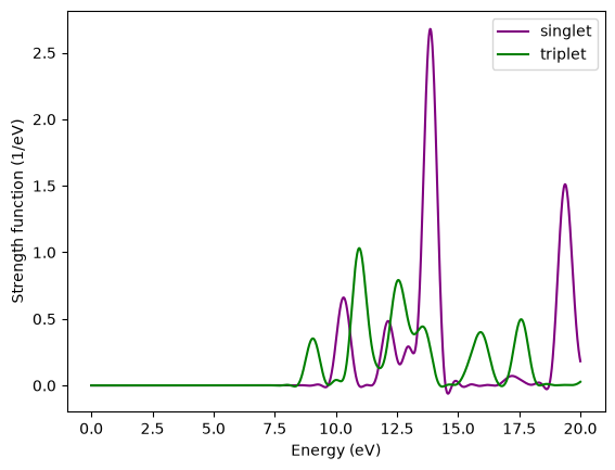
The first triplet transition is found at 9.05 eV, slightly lower energy than the lowest singlet transition.

If you are interested, you can also repeat the calculation for TDDeltaStengthMode = kick_density (the default) and confirm that the result is the same as for the non-spin-polarized calculation.

Using symmetries of non-magnetic systems

As said before, methane is a non-magnetic system, that is, the up and down densities are the same and the magnetization density is zero everywhere:

\[ \rho^{\uparrow}(\mathbf r) = \rho^{\downarrow}(\mathbf r) \]

Note that it is not enough that the total magnetic moment of the system is zero as the previous condition does not hold for anti-ferromagnetic systems. The symmetry in the spin-densities can actually be exploited in order to obtain both the singlet and triplet spectra with a single calculation. This is done by using a special perturbation that is only applied to the spin up states.\(^1\) To use this perturbation, we need to set TDDeltaStrengthMode = kick_spin_and_density. If you repeat the time-propagation with this kick, you should obtain a different cross_section_vector file containing both the singlet and triplet spectra. The singlets are given by StrengthFunction(1) + StrengthFunction(2), while the triplets are given by StrengthFunction(1) - StrengthFunction(2).

Casida equation

The calculation of triplets with the casida mode for spin-polarized systems is currently not implement in Octopus. Nevertheless, just like for the time-propagation, we can take advantage that for non-magnetic systems the two spin are equivalent. In this case it allow us to calculate triplets without the need for a spin-polarized run. The effective kernels in these cases are:

\[f_{\rm Hxc}^{\rm singlet} \left[ \rho \right] = f^{\uparrow}_{\rm Hxc} \left[ \rho ^{\uparrow} \right] + f^{\uparrow}_{\rm Hxc} \left[ \rho^{\downarrow} \right] = f_{\rm H} \left[ \rho \right] + f^{\uparrow}_{\rm xc} \left[ \rho ^{\uparrow} \right] + f^{\uparrow}_{\rm xc} \left[ \rho^{\downarrow} \right]\]

\[f_{\rm Hxc}^{\rm triplet} \left[ \rho \right] = f^{\uparrow}_{\rm Hxc} \left[ \rho ^{\uparrow} \right] - f^{\uparrow}_{\rm Hxc} \left[ \rho^{\downarrow} \right] = f^{\uparrow}_{\rm xc} \left[ \rho ^{\uparrow} \right] - f^{\uparrow}_{\rm xc} \left[ \rho^{\downarrow} \right]\]

Therefore, we start by doing a ground-state and unoccupied states runs exactly as was done in the Optical spectra from Casida tutorial.

!mkdir 5_Triplet_excitations/methane_unnoc/

%%writefile 5_Triplet_excitations/methane_unnoc/inp

stdout = 'stdout_gs_casida.txt'
stderr = 'stderr_gs_casida.txt'

CalculationMode = gs
UnitsOutput = eV_angstrom

Eigensolver = chebyshev_filter
ExtraStates = 4

Radius = 6.5*angstrom
Spacing = 0.24*angstrom

CH = 1.097*angstrom
%Coordinates
 "C" |           0 |          0 |           0
 "H" |  CH/sqrt(3) | CH/sqrt(3) |  CH/sqrt(3)
 "H" | -CH/sqrt(3) |-CH/sqrt(3) |  CH/sqrt(3)
 "H" |  CH/sqrt(3) |-CH/sqrt(3) | -CH/sqrt(3)
 "H" | -CH/sqrt(3) | CH/sqrt(3) | -CH/sqrt(3)
%

Writing 5_Triplet_excitations/methane_unnoc/inp

!cd 5_Triplet_excitations/methane_unnoc/ && octopus

%%writefile 5_Triplet_excitations/methane_unnoc/inp

stdout = 'stdout_unocc_casida.txt'
stderr = 'stderr_unocc_casida.txt'

CalculationMode = unocc
UnitsOutput = eV_angstrom

Radius = 6.5*angstrom
Spacing = 0.24*angstrom

CH = 1.097*angstrom
%Coordinates
 "C" |           0 |          0 |           0
 "H" |  CH/sqrt(3) | CH/sqrt(3) |  CH/sqrt(3)
 "H" | -CH/sqrt(3) |-CH/sqrt(3) |  CH/sqrt(3)
 "H" |  CH/sqrt(3) |-CH/sqrt(3) | -CH/sqrt(3)
 "H" | -CH/sqrt(3) | CH/sqrt(3) | -CH/sqrt(3)
%

ExtraStates = 10

Overwriting 5_Triplet_excitations/methane_unnoc/inp

!cd 5_Triplet_excitations/methane_unnoc/ && octopus

We copy the calculated runs to a separate folder to later reuse the calculated ground-state and unoccupied state for another calculation:

!cp -r 5_Triplet_excitations/methane_unnoc/ 5_Triplet_excitations/casida_triplet/

Then, do a Casida run with the following input file:

%%writefile 5_Triplet_excitations/casida_triplet/inp

stdout = 'stdout_triplet_casida.txt'
stderr = 'stderr_triplet_casida.txt'

CalculationMode = casida
UnitsOutput = eV_angstrom

Radius = 6.5*angstrom
Spacing = 0.24*angstrom

CH = 1.097*angstrom
%Coordinates
 "C" |           0 |          0 |           0
 "H" |  CH/sqrt(3) | CH/sqrt(3) |  CH/sqrt(3)
 "H" | -CH/sqrt(3) |-CH/sqrt(3) |  CH/sqrt(3)
 "H" |  CH/sqrt(3) |-CH/sqrt(3) | -CH/sqrt(3)
 "H" | -CH/sqrt(3) | CH/sqrt(3) | -CH/sqrt(3)
%

ExtraStates = 10

CasidaCalcTriplet = yes

ExperimentalFeatures = yes

Overwriting 5_Triplet_excitations/casida_triplet/inp

!cd 5_Triplet_excitations/casida_triplet && octopus

Once the Casida calculation is finished, run oct-casida_spectrum:

!cd 5_Triplet_excitations/casida_triplet && oct-casida_spectrum

Parser warning: possible mistakes in input file.
List of variable assignments not used by parser:
coordinates[4][3] = -1.196864
coordinates[4][2] = 1.196864
coordinates[4][1] = -1.196864
coordinates[4][0] = "H"
coordinates[3][3] = -1.196864
coordinates[3][2] = -1.196864
coordinates[3][1] = 1.196864
coordinates[3][0] = "H"
coordinates[2][3] = 1.196864
coordinates[2][2] = -1.196864
coordinates[2][1] = -1.196864
coordinates[2][0] = "H"
coordinates[1][3] = 1.196864
coordinates[1][2] = 1.196864
coordinates[1][1] = 1.196864
coordinates[1][0] = "H"
coordinates[0][3] = 0.000000
coordinates[0][2] = 0.000000
coordinates[0][1] = 0.000000
coordinates[0][0] = "C"

For comparison of singlet and triplet we calculate the propgation spectrum as in Optical spectra from Casida tutorial again (you may skip these lines and continue with the plot of you have run the previous tutorials already):

!cp -r --no-target-directory 5_Triplet_excitations/methane_unnoc/ 3_Optical_spectra_from_casida/

%%writefile 3_Optical_spectra_from_casida/inp

stdout = 'stdout_casida.txt'
stderr = 'stderr_casida.txt'

CalculationMode = casida
UnitsOutput = eV_angstrom

Radius = 6.5*angstrom
Spacing = 0.24*angstrom

CH = 1.097*angstrom
%Coordinates
 "C" |           0 |          0 |           0
 "H" |  CH/sqrt(3) | CH/sqrt(3) |  CH/sqrt(3)
 "H" | -CH/sqrt(3) |-CH/sqrt(3) |  CH/sqrt(3)
 "H" |  CH/sqrt(3) |-CH/sqrt(3) | -CH/sqrt(3)
 "H" | -CH/sqrt(3) | CH/sqrt(3) | -CH/sqrt(3)
%

ExtraStates = 10

Overwriting 3_Optical_spectra_from_casida/inp

!cd 3_Optical_spectra_from_casida/ && octopus

!cd 3_Optical_spectra_from_casida/ && oct-casida_spectrum

Parser warning: possible mistakes in input file.
List of variable assignments not used by parser:
coordinates[4][3] = -1.196864
coordinates[4][2] = 1.196864
coordinates[4][1] = -1.196864
coordinates[4][0] = "H"
coordinates[3][3] = -1.196864
coordinates[3][2] = -1.196864
coordinates[3][1] = 1.196864
coordinates[3][0] = "H"
coordinates[2][3] = 1.196864
coordinates[2][2] = -1.196864
coordinates[2][1] = -1.196864
coordinates[2][0] = "H"
coordinates[1][3] = 1.196864
coordinates[1][2] = 1.196864
coordinates[1][1] = 1.196864
coordinates[1][0] = "H"
coordinates[0][3] = 0.000000
coordinates[0][2] = 0.000000
coordinates[0][1] = 0.000000
coordinates[0][0] = "C"

Comparison of absorption spectrum of methane calculated with the Casida equation for singlets and triplets.

We now plot the results of the singlet and the triplet calculation:

fig, ax = plt.subplots()
ax.set_xlabel("Energy (eV)")
ax.set_ylabel("Strength function (1/eV)")

casida_singlet_run = Run("3_Optical_spectra_from_casida/")
casida_triplet_run = Run("5_Triplet_excitations/casida_triplet")

casida_singlet_run.casida.spectrum.casida().plot(
    x="E",
    y="<f>",
    ax=ax,
    label="singlet",
    xlim=[0, 20],
    color="purple",
)

casida_triplet_run.casida.spectrum.casida().plot(
    x="E",
    y="<f>",
    ax=ax,
    label="triplet",
    xlim=[0, 20],
    color="green",
);

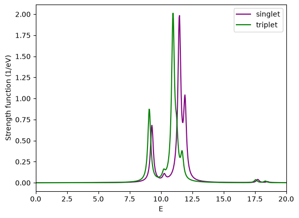
How do the singlet and triplet energy levels compare? Can you explain a general relation between them? How does the run-time compare between singlet and triplet, and why?

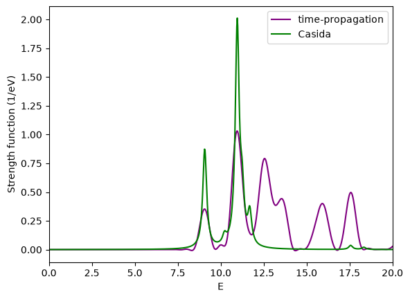
Comparison

As for the singlet spectrum, we can compare the time-propagation and Casida results. What is the main difference, and what is the reason for it?

fig, ax = plt.subplots()
ax.set_xlabel("Energy (eV)")
ax.set_ylabel("Strength function (1/eV)")

triplet_run.td.cross_section_vector().plot(
    x="Energy",
    y="StrengthFunction(1)",
    ax=ax,
    label="time-propagation",
    xlim=[0, 20],
    color="purple",
)


casida_triplet_run.casida.spectrum.casida().plot(
    x="E",
    y="<f>",
    ax=ax,
    label="Casida",
    xlim=[0, 20],
    color="green",
);

References

1. M.J.T. Oliveira, A. Castro, M.A.L. Marques, and A. Rubio, On the use of Neumann’s principle for the calculation of the polarizability tensor of nanostructures, J. Nanoscience and Nanotechnology 8 1-7 (2008);

Tutorial Validation Checks

import numpy as np
from tutorial_helpers.extract_peak import extract_peak

Time propagation

en = triplet_run.td.cross_section_vector()["Energy"]
sf = triplet_run.td.cross_section_vector()["StrengthFunction(1)"]

np.testing.assert_allclose(extract_peak(en, sf, order=1), (10.96, 0.70050, 1.03109), rtol=0.01)

np.testing.assert_allclose(extract_peak(en, sf, order=2), (12.56, 0.77636, 0.79177), rtol=0.01)

Note, the second peak does not correspond to the other Casida peak, but the 5th one does.

np.testing.assert_allclose(extract_peak(en, sf, order=5), (9.06, 0.61739, 0.35271), rtol=0.01)

Casida

en = casida_triplet_run.casida.spectrum.casida()["E"]
sf = casida_triplet_run.casida.spectrum.casida()["<f>"]

np.testing.assert_allclose(extract_peak(en, sf, order=1), (10.96, 0.307361, 2.01191), rtol=0.01)

np.testing.assert_allclose(extract_peak(en, sf, order=2), (9.06, 0.25807, 0.87340), rtol=0.01)