Optical spectra from casida
In this tutorial we will again calculate the absorption spectrum of methane, but this time using Casida’s equations.
import matplotlib.pyplot as plt
from postopus import Run
!mkdir -p 3_Optical_spectra_from_casida
Ground-state
Once again our first step will be the calculation of the ground state. We will use the following input file:
%%writefile 3_Optical_spectra_from_casida/inp

stdout = 'stdout_gs.txt'
stderr = 'stderr_gs.txt'

CalculationMode = gs
UnitsOutput = eV_angstrom

Eigensolver = chebyshev_filter
ExtraStates = 4

Radius = 6.5*angstrom
Spacing = 0.24*angstrom

CH = 1.097*angstrom
%Coordinates
 "C" |           0 |          0 |           0
 "H" |  CH/sqrt(3) | CH/sqrt(3) |  CH/sqrt(3)
 "H" | -CH/sqrt(3) |-CH/sqrt(3) |  CH/sqrt(3)
 "H" |  CH/sqrt(3) |-CH/sqrt(3) | -CH/sqrt(3)
 "H" | -CH/sqrt(3) | CH/sqrt(3) | -CH/sqrt(3)
%
Writing 3_Optical_spectra_from_casida/inp
!cd 3_Optical_spectra_from_casida && octopus
Note that we are using the values for the spacing and radius that were found in the Convergence of the optical spectra tutorial to converge the absorption spectrum.
Unoccupied States
The Casida equation is a (pseudo-)eigenvalue equation written in the basis of particle-hole states. This means that we need both the occupied states – computed in the ground-state calculation – as well as the unoccupied states, that we will now obtain, via a non-self-consistent calculation using the density computed in gs. The input file we will use is
%%writefile 3_Optical_spectra_from_casida/inp

stdout = 'stdout_unocc.txt'
stderr = 'stderr_unocc.txt'

CalculationMode = unocc
UnitsOutput = eV_angstrom

FromScratch = yes

Radius = 6.5*angstrom
Spacing = 0.24*angstrom

CH = 1.097*angstrom
%Coordinates
 "C" |           0 |          0 |           0
 "H" |  CH/sqrt(3) | CH/sqrt(3) |  CH/sqrt(3)
 "H" | -CH/sqrt(3) |-CH/sqrt(3) |  CH/sqrt(3)
 "H" |  CH/sqrt(3) |-CH/sqrt(3) | -CH/sqrt(3)
 "H" | -CH/sqrt(3) | CH/sqrt(3) | -CH/sqrt(3)
%

Eigensolver = chebyshev_filter
ExtraStates = 12
ExtraStatesToConverge = 10
Overwriting 3_Optical_spectra_from_casida/inp
Here we have changed the CalculationMode to unocc and added 10 extra states by setting the ExtraStates input variable.
More precisely, we are using here 12 extra states, and ask to converge only the first 10. This is because the Chebyshev filtering cannot convergence efficiently the last states, so we add here a buffer of two states that we won’t use for Casida calculations. For larger systems, the number of states in the “buffer” needs to be enlarged, such that the wanted states are separated in energy from the last state considered in the calculation.
By running Octopus, we will obtain the first 10 unoccupied states. The solution of the unoccupied states is controlled by the variables in section Eigensolver.
!cd 3_Optical_spectra_from_casida && octopus
We can take a look at the eigenvalues of the unoccupied states in the file static/eigenvalues:
Run("3_Optical_spectra_from_casida").scf.eigenvalues()
| Spin | Eigenvalue | Occupation | Error | |
|---|---|---|---|---|
| st | ||||
| 1 | -- | -16.789494 | 2.0 | ( 4.3E-14) |
| 2 | -- | -9.470218 | 2.0 | ( 9.4E-15) |
| 3 | -- | -9.470218 | 2.0 | ( 8.8E-15) |
| 4 | -- | -9.470218 | 2.0 | ( 1.3E-14) |
| 5 | -- | -0.287589 | 0.0 | ( 1.3E-14) |
| 6 | -- | 0.822694 | 0.0 | ( 1.2E-12) |
| 7 | -- | 0.822694 | 0.0 | ( 4.1E-13) |
| 8 | -- | 0.822694 | 0.0 | ( 1.0E-12) |
| 9 | -- | 1.599660 | 0.0 | ( 3.2E-10) |
| 10 | -- | 1.599660 | 0.0 | ( 9.3E-10) |
| 11 | -- | 1.599660 | 0.0 | ( 4.6E-10) |
| 12 | -- | 1.813361 | 0.0 | ( 4.4E-09) |
| 13 | -- | 1.813361 | 0.0 | ( 1.2E-08) |
| 14 | -- | 2.309013 | 0.0 | ( 8.2E-08) |
| 15 | -- | 3.156972 | 0.0 | ( 3.1E-03) |
| 16 | -- | 3.169228 | 0.0 | ( 1.1E-02) |
As expected, all the wanted state show an error below the threshold (defined by EigensolverTolerance), and the two states in the buffer are not converged.
Casida calculation
We now modify the CalculationMode to casida and rerun Octopus. Note that by default Octopus will use all occupied and unoccupied states that it has available.
Sometimes, it is useful not to use all states. For example, if you have a molecule with 200 atoms and 400 occupied states ranging from -50 to -2 eV, and you are interested in looking at excitations in the visible, you can try to use only the states that are within 10 eV from the Fermi energy. You could select the states to use with CasidaKohnShamStates or CasidaKSEnergyWindow.
As we have only converged 10 extra states, we need to change CasidaKohnShamStates to “1-10” and remove the variables Eigensolver, ExtraStates, and ExtraStatesToConverge.
%%writefile 3_Optical_spectra_from_casida/inp

stdout = 'stdout_casida.txt'
stderr = 'stderr_casida.txt'

CalculationMode = casida
UnitsOutput = eV_angstrom

FromScratch = yes

Radius = 6.5*angstrom
Spacing = 0.24*angstrom

CH = 1.097*angstrom
%Coordinates
 "C" |           0 |          0 |           0
 "H" |  CH/sqrt(3) | CH/sqrt(3) |  CH/sqrt(3)
 "H" | -CH/sqrt(3) |-CH/sqrt(3) |  CH/sqrt(3)
 "H" |  CH/sqrt(3) |-CH/sqrt(3) | -CH/sqrt(3)
 "H" | -CH/sqrt(3) | CH/sqrt(3) | -CH/sqrt(3)
%

CasidaKohnShamStates = "1-10"
Overwriting 3_Optical_spectra_from_casida/inp
!cd 3_Optical_spectra_from_casida && octopus
A new directory will appear named casida, where you can find the file casida/casida:
run = Run("3_Optical_spectra_from_casida")
run.casida.casida()[:10]
| E | <x> | <y> | <z> | <f> | |
|---|---|---|---|---|---|
| 1 | 9.287205 | -8.535608e-03 | -3.473487e-01 | -7.406562e-02 | 1.025495e-01 |
| 2 | 9.287214 | -3.554350e-01 | 9.240746e-03 | -2.368850e-03 | 1.027246e-01 |
| 3 | 9.287970 | -4.301866e-03 | -7.500809e-02 | 3.455168e-01 | 1.015966e-01 |
| 4 | 10.248965 | -2.617820e-03 | 1.444274e-04 | -1.282510e-07 | 6.163610e-06 |
| 5 | 10.250533 | 1.709194e-03 | 1.001594e-04 | 2.237599e-05 | 2.629347e-06 |
| 6 | 10.266320 | 3.416846e-03 | 9.607966e-02 | 5.142273e-02 | 1.067709e-02 |
| 7 | 10.266353 | -1.075059e-01 | 4.442860e-03 | -1.220433e-03 | 1.040001e-02 |
| 8 | 10.266485 | 3.029373e-03 | 4.860678e-02 | -9.856227e-02 | 1.085605e-02 |
| 9 | 10.291095 | -2.027970e-12 | 8.783922e-12 | -2.724241e-12 | 7.985445e-23 |
| 10 | 10.291162 | -2.056627e-03 | -4.775563e-05 | 3.206000e-05 | 3.811281e-06 |
The <x>, <y> and <z> are the transition dipole moments:
where \(\Phi_0\) is the ground state and \(\Phi_I\) is the given excitation. The oscillator strength is given by:
as the average over the three directions. The optical absorption spectrum can be given as the “strength function”, which is
Note that the excitations are degenerate with degeneracy 3. This could already be expected from the \(T_d\) symmetry of methane.
Further information concerning the excitations can be found in the directory casida/casida_excitations. For example, the first excitation at 9.27 eV is analyzed in the file casida/casida_excitations/00001:
# Energy [eV] =    9.28720E+00
# <x> [A] =   -8.53561E-03
# <y> [A] =   -3.47349E-01
# <z> [A] =   -7.40656E-02
           1           5           1   2.4833907312730302E-006
           2           5           1   7.4754734466544639E-002
           3           5           1 -0.50349355151416142
           4           5           1  0.86054549908354638
           1           6           1  -6.4129942312024226E-003
           2           6           1   8.1160643956982442E-003
...
These files contain basically the eigenvector of the Casida equation. The first two columns are respectively the index of the occupied and the index of the unoccupied state, the third is the spin index (always 1 when spin-unpolarized), and the fourth is the coefficient of that state in the Casida eigenvector. This eigenvector is normalized to one, so in this case one can say that 91.7% (0.9582) of the excitation is from state 3 to state 5 (one of 3 HOMO orbitals->LUMO) with small contribution from some other transitions.
Absorption spectrum
To visualize the spectrum, we need to broaden these delta functions with the utility oct-casida_spectrum (run in your working directory, not in casida). It convolves the delta functions with Lorentzian functions. The operation of oct-casida_spectrum is controlled by the variables CasidaSpectrumBroadening (the width of this Lorentzian), CasidaSpectrumEnergyStep, CasidaSpectrumMinenergy, and CasidaSpectrumMaxEnergy. If you run oct-casida_spectrum you obtain the file casida/spectrum.casida. It contains all columns of casida broadened.
!cd 3_Optical_spectra_from_casida && oct-casida_spectrum
Parser warning: possible mistakes in input file.
List of variable assignments not used by parser:
coordinates[4][3] = -1.196864
coordinates[4][2] = 1.196864
coordinates[4][1] = -1.196864
coordinates[4][0] = "H"
coordinates[3][3] = -1.196864
coordinates[3][2] = -1.196864
coordinates[3][1] = 1.196864
coordinates[3][0] = "H"
coordinates[2][3] = 1.196864
coordinates[2][2] = -1.196864
coordinates[2][1] = -1.196864
coordinates[2][0] = "H"
coordinates[1][3] = 1.196864
coordinates[1][2] = 1.196864
coordinates[1][1] = 1.196864
coordinates[1][0] = "H"
coordinates[0][3] = 0.000000
coordinates[0][2] = 0.000000
coordinates[0][1] = 0.000000
coordinates[0][0] = "C"
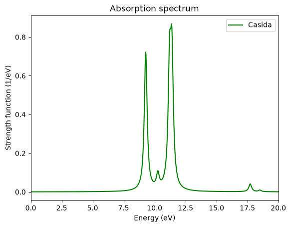
If you are interested in the total absorption spectrum, then you should plot the first and fifth columns:
run = Run("3_Optical_spectra_from_casida")
df_casida = run.casida.spectrum.casida()

fig, ax = plt.subplots()
df_casida.plot(
    x="E",
    y="<f>",
    ax=ax,
    label="Casida",
    color="green",
    xlim=[0, 20],
)
ax.set_title("Absorption spectrum")
ax.set_xlabel("Energy (eV)")
ax.set_ylabel("Strength function (1/eV)");
For comparison of the spectrum obtained via the time-propagation we calculate the propgation spectrum again (as in the Convergence of the optical spectra tutorial, you may skip these lines and continue with the plot if you have run the previous tutorials already):
!cp -r --no-target-directory 3_Optical_spectra_from_casida/ 1_Optical_spectra_from_time_propagation/
%%writefile 1_Optical_spectra_from_time_propagation/inp

stdout = 'stdout_td.txt'
stderr = 'stderr_td.txt'

CalculationMode = td
UnitsOutput = eV_angstrom

Radius = 6.5*angstrom
Spacing = 0.24*angstrom

CH = 1.097*angstrom
%Coordinates
 "C" |           0 |          0 |           0
 "H" |  CH/sqrt(3) | CH/sqrt(3) |  CH/sqrt(3)
 "H" | -CH/sqrt(3) |-CH/sqrt(3) |  CH/sqrt(3)
 "H" |  CH/sqrt(3) |-CH/sqrt(3) | -CH/sqrt(3)
 "H" | -CH/sqrt(3) | CH/sqrt(3) | -CH/sqrt(3)
%

TDPropagator = aetrs
TDTimeStep = 0.0023/eV
TDMaxSteps = 4350  # ~ 10.0/TDTimeStep

TDDeltaStrength = 0.01/angstrom
TDPolarizationDirection = 1
Overwriting 1_Optical_spectra_from_time_propagation/inp
!cd 1_Optical_spectra_from_time_propagation/ && octopus
!cd 1_Optical_spectra_from_time_propagation && oct-propagation_spectrum
time_propagation_run = Run("1_Optical_spectra_from_time_propagation")
df_time_propagation = time_propagation_run.td.cross_section_vector()

fig, ax = plt.subplots()

df_casida.plot(
    x="E",
    y="<f>",
    ax=ax,
    label="Casida",
    color="green",
    xlim=[0, 20],
)

df_time_propagation.plot(
    x="Energy",
    y="StrengthFunction(1)",
    ax=ax,
    label="time-propagation",
    color="purple",
    xlim=[0, 20],
)

ax.set_title("Absorption spectrum")
ax.set_xlabel("Energy (eV)")
ax.set_ylabel("Strength function (1/eV)");
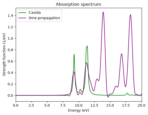
Comparing the spectrum obtained with the time-propagation with the one obtained with the Casida approach using the same grid parameters, we can see that
The peaks of the time-propagation are broader. This can be solved by either increasing the total propagation time, or by increasing the broadening in the Casida approach.
The first two peaks are nearly the same. Probably also the third is OK, but the low resolution of the time-propagation does not allow to distinguish the two close peaks that compose it.
For high energies the spectra differ a lot. The reason is that we only used 10 empty states in the Casida approach. In order to describe better this region of the spectrum we would need more. This is why one should always check the convergence of relevant peaks with respect to the number of empty states.
You probably noticed that the Casida calculation took much less time than the time-propagation. This is clearly true for small or medium-sized systems. However, the implementation of Casida in Octopus has a much worse scaling with the size of the system than the time-propagation, so for larger systems the situation may be different. Note also that in Casida one needs a fair amount of unoccupied states which are fairly difficult to obtain.
If you are interested, you may also compare the Casida results against the Kohn-Sham eigenvalue differences in casida/spectrum.eps_diff and the Petersilka approximation to Casida in casida/spectrum.petersilka.
Tutorial Validation Checks
import numpy as np
from tutorial_helpers.extract_peak import extract_peak
Eigenvalues
ev = Run("3_Optical_spectra_from_casida").scf.eigenvalues()
np.testing.assert_allclose(ev["Eigenvalue"][1], -16.78950, rtol=0.01)
np.testing.assert_allclose(ev["Eigenvalue"][14], 2.30901, rtol=0.01)
Casida calculation
casida_data =Run("3_Optical_spectra_from_casida").casida.casida()
np.testing.assert_allclose(casida_data["E"][1], 9.28719, rtol=0.01)
np.testing.assert_allclose(casida_data["E"][2], 9.28719, rtol=0.01)
np.testing.assert_allclose(casida_data["E"][3], 9.28719, rtol=0.01)
np.testing.assert_allclose(casida_data["E"][4], 10.24907, rtol=0.01)
np.testing.assert_allclose(casida_data["E"][5], 10.24907, rtol=0.01)
Absorption spetrum
casida_spectrum = Run("3_Optical_spectra_from_casida").casida.spectrum.casida()
en = casida_spectrum["E"]
sf = casida_spectrum["<f>"]
np.testing.assert_allclose(extract_peak(en, sf, order=1), (11.37436, 0.4438364622554225, 0.8741958), rtol=0.01)
np.testing.assert_allclose(extract_peak(en, sf, order=2), (9.279082, 0.25696571307408966, 0.7221636), rtol=0.01)