Jellium and jellium slabs

from postopus import Run
import matplotlib.pyplot as plt
from math import pi

In this tutorial, we will compute the ground state of a uniform electron gas, as well as the one of a jellium slab, which is a good model for metallic surfaces.

Jellium

Let us start by performing a calculation for a uniform electrom gas, or jellium. In this tutorial, we choose as an example a Wigner-Seitz radius \(r_s=5.0\). We then create a cubic box with the number of electron corresponding to the density \(n\) given by

\[ \frac{1}{n} = \frac{4}{3}\pi r_s^3 \]

For doing so, we define a constant potential in the box using the Species block, as done in the input file below

mkdir -p 5-jellium/jellium

%%writefile 5-jellium/jellium/inp

stdout = 'stdout_gs.txt'
stderr = 'stderr_gs.txt'

CalculationMode = gs
FromScratch = yes
PeriodicDimensions = 3
BoxShape = parallelepiped

ExperimentalFeatures = yes

aCell = 1.6*angstrom
%LatticeParameters
 aCell | aCell | aCell
 90 | 90 | 90
%

r_s = 5.0 
dens = 1/(4/3*pi*r_s^3)
N_electrons = aCell^3 * dens

%Species
"jellium" | species_user_defined | potential_formula | "dens" | valence | N_electrons
%

%Coordinates
"jellium" | 0 | 0 | 0
%

Spacing = 0.7

Smearing = 0.01*eV
SmearingFunction = fermi_dirac

ExtraStates = 8
Eigensolver = chebyshev_filter

%KPointsGrid
 8 | 8 | 8
%
KPointsUseSymmetries = yes

%Output
  density | axis_z
%

Writing 5-jellium/jellium/inp

!cd 5-jellium/jellium && octopus

We can verify that the resulting density is constant throughout the box.

The expected value of the density is:

\[ \rho = \frac{1}{4/3 \, \pi \, r_s^3} \]

rs = 5.0
1/(4.0/3.0 * pi * rs**3)

0.001909859317102744

The obtained value is:

run_jellium = Run("5-jellium/jellium/")
density_jellium = run_jellium.scf.density().squeeze()
density_jellium.values

array([0.00190986, 0.00190986, 0.00190986, 0.00190986])

Jellium slab

In order to describe a jellium slab, we need to use the special Species call “species_jellium_slab”. This species has two relevant parameters, one is the thickness of the slab, and one is the number of electrons. This is specified as follow:

%Species
"jellium" | species_jellium_slab | thickness | d0 | valence | N_electrons
%

where d_0 and N_electrons are values defined in the input file. As the homogeneous electrons gas are usually parametrized by the Wigner-Seitz radius \(r_s\), the number of electrons in the slab can be defined as

\[ N_e = \frac{A d_0}{\frac{4}{3} \pi r_s^3 } \]

where \(A\) is the area of the slab included in the simulation box.

mkdir -p 5-jellium/jellium-slab

The full input file then reads

%%writefile 5-jellium/jellium-slab/inp

stdout = 'stdout_gs.txt'
stderr = 'stderr_gs.txt'

CalculationMode = gs
FromScratch = yes
PeriodicDimensions = 2
BoxShape = parallelepiped

ExperimentalFeatures = yes

aCell = 1.6*angstrom
%LatticeParameters
 aCell | aCell | 25*angstrom
 90 | 90 | 90
%

r_s = 5.0 
d0 = 16.0*angstrom
N_electrons = aCell^2 * d0 / (4/3*pi*r_s^3)  

%Species
"jellium" | species_jellium_slab | thickness | d0 | valence | N_electrons
%

%Coordinates
"jellium" | 0 | 0 | 0
%

Spacing = 0.7

Smearing = 0.01*eV
SmearingFunction = fermi_dirac

ExtraStates = 4
Eigensolver = chebyshev_filter

%KPointsGrid
 12 | 12 | 1
%
KPointsUseSymmetries = yes

%Output
 density | axis_z
%

Writing 5-jellium/jellium-slab/inp

!cd 5-jellium/jellium-slab && octopus

Here, we used a unit cell of \(1.6\unicode{x212B}\times1.6\unicode{x212B}\) in-plane size, and a size along the perpendicular direction of \(25 \unicode{x212B}\). We then a jellium slab of thickness \(16 \unicode{x212B}\), centered here around \(z=0\), with \(r_s=5\), which correspond to 0.5279 electrons in the system. Because of the fractional occupations, and because we describe a metallic surface, we employed here a small Smearing of 10 meV, with a Fermi-Dirac distribution.

After running this input file, one can plot the density of the jellium slab.

from postopus import Run

run = Run('5-jellium/jellium-slab')
density = run.scf.density()

rs = 5.0
rho = 1/(4.0/3.0*pi*(rs**3))
Lz = 30.2356/2

fig, axs = plt.subplots()
density.plot(ax=axs)
axs.plot([-Lz, -Lz, Lz, Lz], [0, rho, rho, 0], color="black")
axs.set_title("Electron density of the jellium slab, compared to the profile of the uniform background density (black lines).");

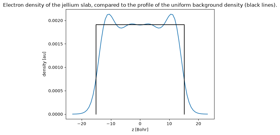
Clear Friedel oscillations of the electron density near the surface are observed, and the result can be compared to the result obtained by Lang and Kohn, see Fig. 2 in Ref.\(^1\).

References

1. N. D. Lang and W. Kohn, Theory of Metal Surfaces: Charge Density and Surface Energy, Phys. Rev. B, 1 4555 (1970)

Tutorial Validation Checks

import numpy as np
from tutorial_helpers.extract_peak import extract_peak

np.testing.assert_allclose(run.scf.info.get_total_energy(), 1.89212707, rtol=0.001)

np.testing.assert_allclose(density_jellium, rho, rtol=0.001)

np.testing.assert_allclose(density.sel(z=0).values[0], 0.0019013674451981, rtol=0.001)

np.testing.assert_allclose(density.sel(z=16.1).values[0], 0.000406479719693468, rtol=0.001)