Particle in a box

In the previous tutorial, we considered applying a user-defined potential. What if we wanted to do the classic quantum problem of a particle in a box, “i.e.” an infinite square well?

\[ V(x)= \begin{cases} 0, & -\frac{L}{2} < x < \frac{L}{2} \cr \infty, & \text{otherwise} \end{cases} \]

There is no meaningful way to set an infinite value of the potential for a numerical calculation. However, we can instead use the boundary conditions to set up this problem. In the locations where the potential is infinite, the wavefunctions must be zero. Therefore, it is equivalent to solve for an electron in the potential above in all space, or to solve for an electron just in the domain \( x \in [-\tfrac{L}{2}, \tfrac{L}{2}]\) with zero boundary conditions on the edges. In the following input file, we can accomplish this by setting the “radius” to \(\tfrac{L}{2}\)​, for the default box shape of “sphere” which means a line in 1D.

import matplotlib.pyplot as plt
import numpy as np
from postopus import Run

!mkdir -p 3-particle-in-a-box

Input

As usual, we will need to write an input file describing the system we want to calculate:

%%writefile 3-particle-in-a-box/inp

stdout = 'stdout_gs.txt'
stderr = 'stderr_gs.txt'

FromScratch = yes
CalculationMode = gs

Dimensions = 1
TheoryLevel = independent_particles

L = 10
Radius = L/2
Spacing = 0.01

%Species
  "null" | species_user_defined | potential_formula | "0" | valence | 1
%

%Coordinates
  "null" | 0
%

LCAOStart = lcao_states

%Output
  wfs
%
OutputFormat = axis_x

Writing 3-particle-in-a-box/inp

Run this input file and look at the ground-state energy and the eigenvalue of the single state.

!cd 3-particle-in-a-box && octopus

run = Run("3-particle-in-a-box")

run.scf.info.get_total_energy()

0.05003035

run.scf.info.get_eigenvalues()

	Spin	Eigenvalue	Occupation
st
1	--	0.050030	1.0
2	--	0.196926	0.0

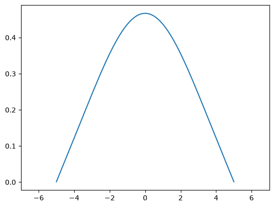
Now we can look at the wave function of the lowest state:

wf = run.default.scf.wf().isel(step=-1).sel(st=1)
plt.plot(wf.x, wf.real)
plt.xlim(min(wf.x) - 2, max(wf.x) + 2);

Exercises

• Calculate unoccupied states and check that they obey the expected relation.

%%writefile 3-particle-in-a-box/inp

stdout = 'stdout_unocc.txt'
stderr = 'stderr_unocc.txt'

FromScratch = yes
CalculationMode = unocc

Dimensions = 1
TheoryLevel = independent_particles

L = 10
Radius = L/2
Spacing = 0.01

%Species
  "null" | species_user_defined | potential_formula | "0" | valence | 1
%

%Coordinates
  "null" | 0
%

LCAOStart = lcao_states
extrastates = 10

%Output
  wfs
%
OutputFormat = axis_x

Overwriting 3-particle-in-a-box/inp

!cd 3-particle-in-a-box && octopus

# Analytical solution
def make_psi(n, L):
    def psi_n_l(x):
        return -((2 / L) ** 0.5) * np.sin(n * np.pi / L * (x + L / 2))

    return psi_n_l

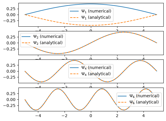
• Plot the wavefunctions and compare to your expectation.

run = Run("./3-particle-in-a-box/")
wfs = run.scf.wf().isel(step=-1)
states = [1, 2, 4, 6]

fig, axs = plt.subplots(len(states))
for i, state in enumerate(states):
    wf = wfs.sel(st=state).squeeze()
    axs[i].plot(wf.x, wf.real, label=fr"$\Psi_{state}$ (numerical)")
interval = (wfs.x.min().item(), wfs.x.max().item())
L = interval[1] - interval[0]
x = np.linspace(interval[0], interval[1])
for i, n in enumerate(states):
    psi_n = make_psi(n, L)
    axs[i].plot(x, psi_n(x), label=fr"$\Psi_{n}$ (analytical)", linestyle="--")
    axs[i].legend()

Further exercises

• Vary the box size and check that the energy has the correct dependence.

• Set up a calculation of a ‘‘finite’’ square well and compare results to the infinite one as a function of potential step. (Hint: along with the usual arithmetic operations, you may also use logical operators to create a piecewise-defined expression. See Input file).

• Try a 2D or 3D infinite square well.

Tutorial Validation Checks

import numpy as np

np.testing.assert_allclose(run.scf.info.get_total_energy(), 0.05003052, rtol=0.001)

np.testing.assert_allclose(run.scf.info.get_eigenvalues()['Eigenvalue'].to_numpy(), [0.050031, 0.196926], rtol=0.001)