1D Helium
The next example will be the helium atom in one dimension which also has two electrons, just as we used for the harmonic oscillator. The main difference is that instead of describing two electrons in one dimension we will describe one electron in two dimensions. The calculation in this case is not a DFT one, but an exact solution of the Schrödinger equation — not an exact solution of the helium atom, however, since it is a one-dimensional model.
Equivalence between two 1D electrons and one 2D electron
To show that we can treat two electrons in one dimension as one electron in two dimensions, lets start by calling \(x\,\) and \(y\,\) the coordinates of the two electrons. The Hamiltonian would be (note that the usual Coulomb interaction between particles is usually substituted, in 1D models, by the soft Coulomb potential, \(u(x)=(1+x^2)^{(-1/2)}\,\)):
Instead of describing two electrons in one dimension, however, we may very well think of one electron in two dimensions, subject to a external potential with precisely the shape given by:
Since the Hamiltonian is identical, we will get the same result. Whether we regard \(x\,\) and \(y\,\) as the coordinates of two different particles in one dimension or as the coordinates of the same particle along the two axes in two dimensions is entirely up to us. (This idea can actually be generalized to treat two 2D particles via a 4D simulation in Octopus too!) Since it is usually easier to treat only one particle, we will solve the one-dimensional helium atom in two dimensions. We will also therefore get a “two-dimensional wave-function”. In order to plot this wave-function we specify an output plane instead of an axis.
from matplotlib import cm
import matplotlib.pyplot as plt
from postopus import Run
!mkdir -p 4-1d-helium
Input
With the different potential and one more dimension the new input file looks like the following
%%writefile 4-1d-helium/inp

stdout = 'stdout_gs.txt'
stderr = 'stderr_gs.txt'

CalculationMode = gs

Dimensions = 2
TheoryLevel = independent_particles

BoxShape = parallelepiped
Lsize = 8
Spacing = 0.1

%Output
  wfs | plane_z
%

%Species
 "helium" | species_user_defined | potential_formula | "-2/(1+x^2)^(1/2)-2/(1+y^2)^(1/2)+1/(1+(x-y)^2)^(1/2)" | valence | 1
%

%Coordinates
 "helium"| 0 | 0
%
Writing 4-1d-helium/inp
For more information on how to write a potential formula expression, see Input file.
We named the species “helium” instead of “He” because “He” is already the name of a pseudopotential for the actual 3D helium atom.
Running
The calculation should converge within 14 iterations. As usual, the results are summarized in the static/info file, where you can find
!cd 4-1d-helium && octopus
**************************** Theory Level ****************************
Input: [TheoryLevel = independent_particles]
**********************************************************************

SCF converged in   34 iterations

Some of the states are not fully converged!
Eigenvalues [H]
 #st  Spin   Eigenvalue      Occupation
   1   --    -2.238257       1.000000
   2   --    -1.808290       0.000000

Energy [H]:
      Total       =        -2.23825730
      Free        =        -2.23825730
      -----------
      Ion-ion     =         0.00000000
      Eigenvalues =        -2.23825730
      Hartree     =         0.00000000
      Int[n*v_xc] =         0.00000000
      Exchange    =         0.00000000
      Correlation =         0.00000000
      vanderWaals =         0.00000000
      Delta XC    =         0.00000000
      Entropy     =         1.38629436
      -TS         =        -0.00000000
      Photon ex.  =         0.00000000
      Kinetic     =         0.28972499
      External    =        -2.52798228
      Non-local   =         0.00000000
      Int[n*v_E]  =         0.00000000

Dipole:                 [b]          [Debye]
      <x> =    6.76728E-09      1.72007E-08
      <y> =    5.61858E-08      1.42810E-07

Convergence:
      abs_energy =  9.92539384E-13 ( 0.00000000E+00) [H]
      rel_energy =  4.43442935E-13 ( 0.00000000E+00)
      abs_dens =  4.85939638E-07 ( 0.00000000E+00)
      rel_dens =  4.85939638E-07 ( 1.00000000E-06)
      abs_evsum =  9.92539384E-13 ( 0.00000000E+00) [H]
      rel_evsum =  4.43442935E-13 ( 0.00000000E+00)
As we are running with non-interacting electrons, the Hartree, exchange and correlation components of the energy are zero. Also the ion-ion term is zero, as we only have one “ion”.
Unoccupied States
Now you can do just the same thing we did for the harmonic oscillator and change the unoccupied calculation mode:
%%writefile 4-1d-helium/inp
CalculationMode = unocc

stdout = 'stdout_unocc.txt'
stderr = 'stderr_unocc.txt'

Dimensions = 2
TheoryLevel = independent_particles

BoxShape = parallelepiped
Lsize = 8
Spacing = 0.1

%Output
  wfs | plane_z
%
OutputWfsNumber = "1-4,6"

%Species
 "helium" | species_user_defined | potential_formula | "-2/(1+x^2)^(1/2)-2/(1+y^2)^(1/2)+1/(1+(x-y)^2)^(1/2)" | valence | 1
%

%Coordinates
 "helium"| 0 | 0
%

ExtraStates = 5
Overwriting 4-1d-helium/inp
!cd 4-1d-helium && octopus
We have added extra states and also restricted the wavefunctions to plot (OutputWfsNumber = “1-4,6”).
The results of this calculation can be found in the file static/eigenvalues . In this case it looks like
run = Run("4-1d-helium")
run.scf.eigenvalues()
| Spin | Eigenvalue | Occupation | Error | |
|---|---|---|---|---|
| st | ||||
| 1 | -- | -2.238257 | 1.0 | ( 2.5E-13) |
| 2 | -- | -1.815718 | 0.0 | ( 9.4E-07) |
| 3 | -- | -1.701548 | 0.0 | ( 5.5E-04) |
| 4 | -- | -1.629239 | 0.0 | ( 1.2E-03) |
| 5 | -- | -1.608656 | 0.0 | ( 8.5E-05) |
| 6 | -- | -1.497847 | 0.0 | ( 2.2E-01) |
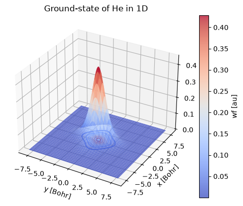
Apart from the eigenvalues and occupation numbers we asked Octopus to output the wave-functions. To plot them, we will use postopus.
wf = run.scf.wf().squeeze()
st = wf.sel(st=1)
st.plot.surface(cmap=cm.coolwarm, alpha=0.75)
st.plot.contour(offset=0, cmap=cm.coolwarm)

plt.title("Ground-state of He in 1D");
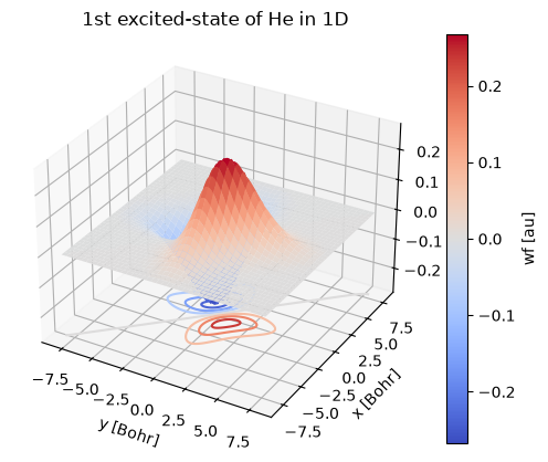
st = wf.sel(st=2)
st.plot.surface(cmap=cm.coolwarm)
st.plot.contour(offset=st.min(), cmap=cm.coolwarm)

plt.title("1st excited-state of He in 1D");
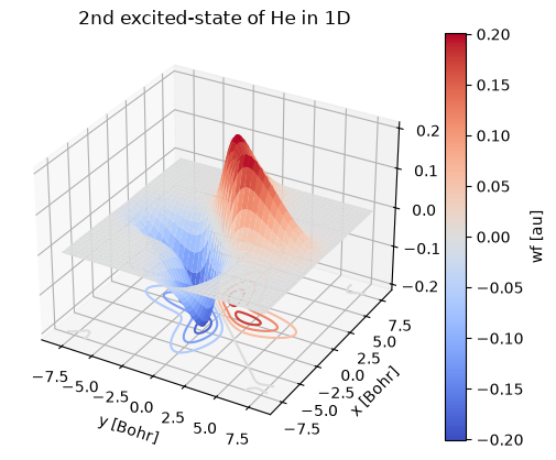
st = wf.sel(st=3)
st.plot.surface(cmap=cm.coolwarm)
st.plot.contour(offset=st.min(), cmap=cm.coolwarm)

plt.title("2nd excited-state of He in 1D");
Exercises
Calculate the helium atom in 1D, assuming that the 2 electrons of helium do not interact using Dimensions = 1. Can you justify the differences?
See how the results change when you change the interaction. Often one models the Coulomb interaction by \(1/\sqrt{a^2+r^2}\,\), and fits the parameter \(a\,\) to reproduce some required property.
Tutorial Validation Checks
from tutorial_helpers.extract_peak import extract_peak
import numpy as np
st_1 = wf.sel(st=1)
np.testing.assert_allclose(extract_peak(st_1.sel(y=0)['x'].to_numpy(), st_1.sel(y=0).to_numpy(), order=1),
                           (0.0, 3.0289409027832606, 0.446356903867646), rtol=0.001)
np.testing.assert_allclose(extract_peak(st_1.sel(y=0)['x'].to_numpy(), st_1.sel(y=2).to_numpy(), order=1),
                           (-0.2, 2.58603004705669, 0.152696387585338), rtol=0.001)
st_2 = wf.sel(st=2)
np.testing.assert_allclose(extract_peak(st_2.sel(y=0)['x'].to_numpy(), st_2.sel(y=0).to_numpy(), order=1),
                           (-1.6, 3.344030982764739, 0.215928032717159), rtol=0.001)
np.testing.assert_allclose(extract_peak(st_2.sel(y=0)['x'].to_numpy(), st_2.sel(y=2).to_numpy(), order=1),
                           (-0.4, 2.7869107494894805, 0.230792905667217), rtol=0.001)