Kohn-Sham inversion

from postopus import Run

Thanks to the mapping between the electronic density and the Kohn-Sham potential it is possible to compute the exchange-correlation (xc) potential from the sole knowledge of the density. The usual SCF cycle of a ground-state calculation aims at finding the ground state density by iteratively updating the Hartree and xc potential. However, it is also possible to fix the density and ask the question: what is the xc potential that would produce this density, knowing the external potential acting on the electrons. The procedure that finds this xc potential is known as the Kohn-Sham inversion. This has been extensively used to learn about the exact xc potential for systems in which the exact density is known or where higher theory level can produce high-quality reference densities.

In this tutorial, we will explore how to perform the Kohn-Sham inversion for the simplest case: a one dimensional system with two electrons occupying the same orbital. In this case, the analytical expression of the xc potential is known. For more than two electrons, one needs to use iterative schemes, that we won’t discuss in this tutorial.

Input for the reference density

As usual, we will need to write an input file describing the system we want to calculate. In order to perform the Kohn-Sham inversion, we need first a density. Here, we will use Hartree-Fock theory to evaluate the ground-state of a 1D soft-Coulomb hydrogen atom.

mkdir -p 2-kohn-sham-inversion/density

%%writefile 2-kohn-sham-inversion/density/inp

stdout = 'stdout_gs.txt'
stderr = 'stderr_gs.txt'

CalculationMode = gs
FromScratch = yes

Dimensions = 1

BoxShape = parallelepiped
%Lsize
 15
%
Spacing = 0.05

%Species
'He1D' | species_soft_coulomb | softening | 1 | valence | 2
%

%Coordinates
'He1D' | 0.0
%

TheoryLevel = hartree_fock
AdaptivelyCompressedExchange = yes
ExperimentalFeatures = yes

%Output
 density | axis_x
%

ConvRelDens = 1e-8
EigensolverMaxIter = 50
ExtraStates = 2
ExtraStatesToConverge = 1

Writing 2-kohn-sham-inversion/density/inp

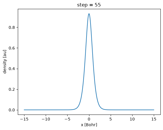
Running this input file will produce the file static/density.y=0,z=0. This is the density we will use in order to perform the Kohn-Sham inversion and find the local xc potential that produces it.

!cd 2-kohn-sham-inversion/density && octopus

run_dens = Run("2-kohn-sham-inversion/density/")
density = run_dens.scf.density()
density.plot()

[<matplotlib.lines.Line2D at 0x7f62793ae5d0>]

The eigenvalues are:

run_dens.scf.info.get_eigenvalues()

	Spin	Eigenvalue	Occupation
st
1	--	-0.750249	2.0
2	--	0.051642	0.0
3	--	0.055209	0.0

Kohn-Sham inversion

The Kohn-Shame inversion is done using the following input file.

mkdir -p 2-kohn-sham-inversion/inversion

!cp -r 2-kohn-sham-inversion/density/static/density.y=0,z=0 2-kohn-sham-inversion/inversion/density-inp.y=0,z=0

%%writefile 2-kohn-sham-inversion/inversion/inp

stdout = 'stdout_inv.txt'
stderr = 'stderr_inv.txt'

CalculationMode = invert_ks
FromScratch = yes

ExperimentalFeatures = yes

Dimensions = 1

BoxShape = parallelepiped
%Lsize
 15
%
Spacing = 0.05

%Species
'He1D' | species_soft_coulomb | softening | 1 | valence | 2
%

%Coordinates
'He1D' | 0.0
%

XCFunctional = ks_inversion

InvertKSTargetDensity = "density-inp.y=0,z=0"
InvertKSmethod = two_particle

%Output
 potential | axis_x
 density | axis_x
%

Writing 2-kohn-sham-inversion/inversion/inp

We first note that here we change the CalculationMode to be invert_ks instead of gs. Other changes are mandatory. We need to set XCFunctional to ks_inversion. Then, we need to instruct the code where to find the target density. This is specified thanks to the variable InvertKSTargetDensity. Importantly, whereas here we produced the target density using Octopus, with the same grid, there is no requirement on the grid in which the data is provided. If the grid is different, Octopus will perform internally an interpolation to obtain the density on the desired grid.

Finally, we need to choose the methodology used for the Kohn-Sham inversion. As in the present case we are considering the two-electron in one orbital case, we have set InvertKSmethod to two_particle.

!cd 2-kohn-sham-inversion/inversion && octopus

from postopus import Run
import matplotlib.pyplot as plt

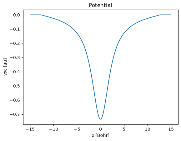
run = Run("2-kohn-sham-inversion/inversion")
run.scf.vxc().plot()
plt.title("Potential");

Comparison with the slater potential

In the first step of this tutorial, we performed a Hartree-Fock calculation in order to produce the target density. This is a nonlocal theory and in general the only way to obtain the corresponding local potential would be via the solution of the OEP equation. This can be done by Octopus. However, in our case, as we have a single orbital occupied, we know the analytical solution. This is the Slater potential.

We can therefore perform a Koh-Sham DFT calculation for our system using the following the input file.

mkdir -p 2-kohn-sham-inversion/slater

%%writefile 2-kohn-sham-inversion/slater/inp

stdout = 'stdout_gs.txt'
stderr = 'stderr_gs.txt'

CalculationMode = gs
FromScratch = yes

Dimensions = 1

BoxShape = parallelepiped
%Lsize
 15
%
Spacing = 0.05

%Species
'He1D' | species_soft_coulomb | softening | 1 | valence | 2
%

%Coordinates
'He1D' | 0.0   
%

XCFunctional = slater_x

%Output
 potential | axis_x
 density | axis_x
%

ConvRelDens = 1e-8
EigensolverMaxIter = 50
ExtraStates = 2
ExtraStatesToConverge = 1

Writing 2-kohn-sham-inversion/slater/inp

!cd 2-kohn-sham-inversion/slater && octopus

This calculation produces the same eigenvalue and density as the original HF calculation. We can finally compare the Slater potential and the one obtained from the Kohn-Sham inversion. There are few points to note:

• The Kohn-Sham inversion potential is shifted upwards

• It goes exactly at zero close to the box edges

run_slater = Run("2-kohn-sham-inversion/slater")

fix, ax = plt.subplots()
run.scf.vxc()[-1].plot(ax=ax, label='Inversion')
run_slater.scf.vxc()[-1].plot(ax=ax, label='Slater')
plt.title("Potential")
plt.legend();

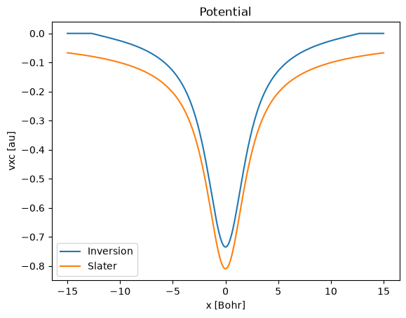
These two points are related to the treatment of the asymptotic part of the potential and are limitations of the current implementation. To prevent numerical noise, the current implementation sets to zero the points where the density is too samll. As the xc potential can be defined up to a constant, this freedom is used to avoid discontinuity of the potential where we set it to zero.

Note, that the eigenvalue of the occupied state is reproduced exactly. This is not the case for the unoccupied states.

run_slater.scf.info.get_eigenvalues()

	Spin	Eigenvalue	Occupation
st
1	--	-0.750249	2.0
2	--	-0.256559	0.0
3	--	-0.142115	0.0

By shifting the result of the Kohn-Sham inversion, we find that this matches perfectly the Slater potential. However, one can employ the fact that the interaction is a soft-Coulomb potential. This allows for an analytical treatment of the asymptotic region. This is done using the variable KSInversionAsymptotics to xc_asymptotics_sc. If you rerun the Kohn-Sham inversion with this method, you should now properly reproduce perfectly the Slater potential.

Tutorial Validation Checks

from postopus import Run
import numpy as np
from tutorial_helpers.extract_peak import extract_peak

Reference density

density = run.scf.density()

last_dens = density[-1]

np.testing.assert_allclose(extract_peak(last_dens['x'].to_numpy(), last_dens.to_numpy(), order=1), (0.0, 1.8931844073188755, 0.931127246983921), rtol=0.001)

Inversion potential

pot = run.scf.vxc()

np.testing.assert_allclose(extract_peak(pot['x'].to_numpy(), -pot[-1].to_numpy(), order=1), (0.0, 4.559799503442996, 0.734672997816137), rtol=0.001)

Slater

run_slater = Run("2-kohn-sham-inversion/slater/")

np.testing.assert_allclose(run_slater.scf.info.get_total_energy(),-2.22420955, rtol=0.001)

np.testing.assert_allclose(run_slater.scf.info.get_eigenvalues()['Eigenvalue'].values[0],
                           run_dens.scf.info.get_eigenvalues()['Eigenvalue'].values[0], rtol=0.001)