Navigation :
Manual
Input Variables
Tutorials
-
Octopus Basics
-
Optical Response
-
Model Systems
-
Multisystem
-
Periodic Systems
-
Maxwell Systems
-- Maxwell overview
-- Maxwell input file
-- Cosinoidal plane wave in vacuum
-- Interference of two cosinoidal plane waves
-- Cosinoidal plane wave hitting a linear medium box
-- Gaussian-shaped external current density
-- Creating geometries
-- Simulation box
-
Unsorted tutorials
-
Courses
Developers
Releases
Gaussian-shaped external current density
Gaussian-shaped external current density passed by a Gaussian temporal current pulse
No absorbing boundaries
click for complete input
# ----- Calculation mode and parallelization ------------------------------------------------------

 CalculationMode   = td
 RestartWrite = no
 ExperimentalFeatures = yes

%Systems
  'Maxwell' | maxwell
%

 Maxwell.ParDomains = auto
 Maxwell.ParStates  = no

# ----- Maxwell box variables ---------------------------------------------------------------------

 # free maxwell box limit of 10.0

 lsize_mx = 10.0
 dx_mx    = 0.5

 Maxwell.BoxShape   = parallelepiped

 %Maxwell.Lsize
  lsize_mx | lsize_mx | lsize_mx
 %

 %Maxwell.Spacing
  dx_mx | dx_mx | dx_mx
 %

# ----- Maxwell calculation variables -------------------------------------------------------------

 MaxwellHamiltonianOperator = faraday_ampere

 %MaxwellBoundaryConditions
  zero | zero | zero
 %

 %MaxwellAbsorbingBoundaries
  not_absorbing | not_absorbing | not_absorbing
 %

# ----- Output variables --------------------------------------------------------------------------

 OutputFormat = axis_x + axis_y + axis_z + plane_x + plane_y + plane_z


# ----- Maxwell output variables ------------------------------------------------------------------

 %MaxwellOutput
  electric_field
  magnetic_field
  maxwell_energy_density
  trans_electric_field
 %

 MaxwellOutputInterval = 10
 MaxwellTDOutput       = maxwell_energy + maxwell_total_e_field

 %MaxwellFieldsCoordinate
   0.00 | 0.00 | 0.00
 %


# ----- Time step variables -----------------------------------------------------------------------

 TDSystemPropagator = exp_mid
 timestep             = 1 / ( sqrt(c^2/dx_mx^2 + c^2/dx_mx^2 + c^2/dx_mx^2) )
 TDTimeStep           = timestep
 TDPropagationTime    = 180 * timestep

# Maxwell field variables

# ----- External current ------------------------------------------------------------------------

 ExternalCurrent = yes
 t1 = 4 * 5.0 / c
 t2 = 6 * 5.0 / c
 tw = 0.03
 j = 1.0000

 %UserDefinedMaxwellExternalCurrent
   current_td_function | "0" | "0" | "j*exp(-x^2/2)*exp(-y^2/2)*exp(-z^2/2)" | 0 | "env_func_1"
   current_td_function | "0" |" 0" | "j*exp(-x^2/2)*exp(-y^2/2)*exp(-z^2/2)" | 0 | "env_func_2"
 %

 %TDFunctions
   "env_func_1" | tdf_gaussian |  1.0 | tw | t1
   "env_func_2" | tdf_gaussian | -1.0 | tw | t2
 %
Instead of an incoming external plane wave, Octopus can simulate also external current
densities placed inside the simulation box. In this example we place one shape of such
a current density in the simulation box
 %MaxwellBoundaryConditions
  zero | zero | zero
 %

 %MaxwellAbsorbingBoundaries
  not_absorbing | not_absorbing | not_absorbing
 %
Since we start with no absorbing boundaries, we reset the box size to 10.0.
# ----- Maxwell box variables ---------------------------------------------------------------------

 # free maxwell box limit of 10.0

 lsize_mx = 10.0
 dx_mx    = 0.5

 Maxwell.BoxShape   = parallelepiped

 %Maxwell.Lsize
  lsize_mx | lsize_mx | lsize_mx
 %

 %Maxwell.Spacing
  dx_mx | dx_mx | dx_mx
 %
The external current density is switched on by the corresponding options and
two blocks define its spatial distribution and its temporal behavior. The
spatial distribution of our example external current is a Gaussian distribution
in 3D. The temporal pulse is one Gaussian along the y-axis and one along the
opposite direction but time shifted.
# ----- External current ------------------------------------------------------------------------

 ExternalCurrent = yes
 t1 = 4 * 5.0 / c
 t2 = 6 * 5.0 / c
 tw = 0.03
 j = 1.0000

 %UserDefinedMaxwellExternalCurrent
   current_td_function | "0" | "0" | "j*exp(-x^2/2)*exp(-y^2/2)*exp(-z^2/2)" | 0 | "env_func_1"
   current_td_function | "0" |" 0" | "j*exp(-x^2/2)*exp(-y^2/2)*exp(-z^2/2)" | 0 | "env_func_2"
 %

 %TDFunctions
   "env_func_1" | tdf_gaussian |  1.0 | tw | t1
   "env_func_2" | tdf_gaussian | -1.0 | tw | t2
 %
gnuplot script
set pm3d
set view map
set palette defined (-0.005 "blue", 0 "white", 0.005"red")
set term png size 1000,500

unset surface
unset key

set output 'plot1.png'

set xlabel 'x-direction'
set ylabel 'y-direction'
set cbrange [-0.005:0.005]

set multiplot

set origin 0.025,0
set size 0.45,0.9
set size square
set title 'Electric field E_z (t=0.252788 au)'
sp [-10:10][-10:10][-0.01:0.01] 'Maxwell/output_iter/td.0000120/e_field-z.z=0' u 1:2:3

set origin 0.525,0
set size 0.45,0.9
set size square
set title 'Electric field E_z (t=0.379182 au)'
sp [-10:10][-10:10][-0.01:0.01] 'Maxwell/output_iter/td.0000180/e_field-z.z=0' u 1:2:3

unset multiplot
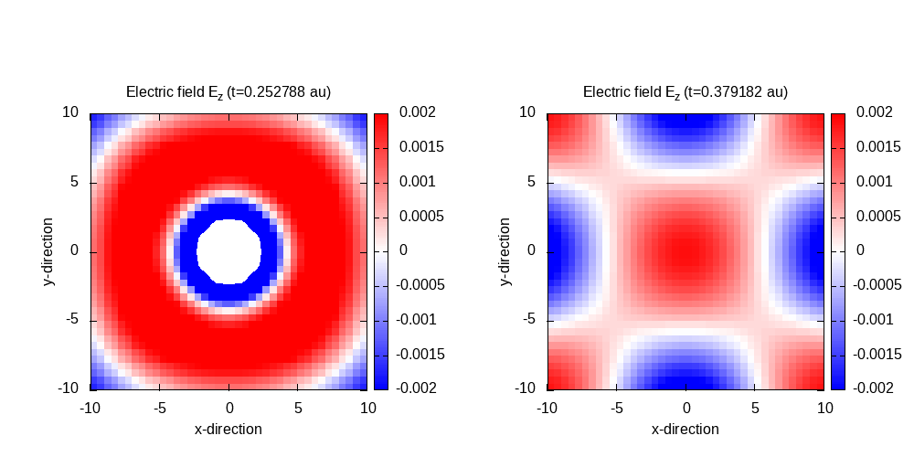
Contour plot of the electric field in z-direction after 120 time steps for
t=0.24 and 180 time steps for t=0.36:
Mask absorbing boundaries
click for complete input
# ----- Calculation mode and parallelization ------------------------------------------------------

 CalculationMode   = td
 RestartWrite = no
 ExperimentalFeatures = yes

%Systems
  'Maxwell' | maxwell
%

 Maxwell.ParDomains = auto
 Maxwell.ParStates  = no

# ----- Maxwell box variables ---------------------------------------------------------------------

 # free maxwell box limit of 10.0 plus 5.0 for absorbing boundary conditions

 lsize_mx = 15.0
 dx_mx    = 0.5

 Maxwell.BoxShape   = parallelepiped

 %Maxwell.Lsize
  lsize_mx | lsize_mx | lsize_mx
 %

 %Maxwell.Spacing
  dx_mx | dx_mx | dx_mx
 %

# ----- Maxwell calculation variables -------------------------------------------------------------

 MaxwellHamiltonianOperator = faraday_ampere

 %MaxwellBoundaryConditions
  zero | zero | zero
 %

 %MaxwellAbsorbingBoundaries
  mask | mask | mask
 %

 MaxwellABWidth = 5.0

# ----- Output variables --------------------------------------------------------------------------

 OutputFormat = axis_x + axis_y + axis_z + plane_x + plane_y + plane_z


# ----- Maxwell output variables ------------------------------------------------------------------

 %MaxwellOutput
  electric_field
  magnetic_field
  maxwell_energy_density
  trans_electric_field
 %

 MaxwellOutputInterval = 10
 MaxwellTDOutput       = maxwell_energy + maxwell_total_e_field

 %MaxwellFieldsCoordinate
   0.00 | 0.00 | 0.00
 %


# ----- Time step variables -----------------------------------------------------------------------

 TDSystemPropagator = exp_mid
 timestep             = 1 / ( sqrt(c^2/dx_mx^2 + c^2/dx_mx^2 + c^2/dx_mx^2) )
 TDTimeStep           = timestep
 TDPropagationTime    = 180 * timestep

# Maxwell field variables

# ----- External current ------------------------------------------------------------------------

 ExternalCurrent = yes
 t1 = 4 * 5.0 / c
 t2 = 6 * 5.0 / c
 tw = 0.03
 j = 1.0000

 %UserDefinedMaxwellExternalCurrent
   current_td_function | "0" | "0" | "j*exp(-x^2/2)*exp(-y^2/2)*exp(-z^2/2)" | 0 | "env_func_1"
   current_td_function | "0" |" 0" | "j*exp(-x^2/2)*exp(-y^2/2)*exp(-z^2/2)" | 0 | "env_func_2"
 %

 %TDFunctions
   "env_func_1" | tdf_gaussian |  1.0 | tw | t1
   "env_func_2" | tdf_gaussian | -1.0 | tw | t2
 %
We can add now mask absorbing boundaries.
 %MaxwellBoundaryConditions
  zero | zero | zero
 %

 %MaxwellAbsorbingBoundaries
  mask | mask | mask
 %

 MaxwellABWidth = 5.0
Accordingly to the additional absorbing width, we have to update the simulation
box dimensions.
# ----- Maxwell box variables ---------------------------------------------------------------------

 # free maxwell box limit of 10.0 plus 5.0 for absorbing boundary conditions

 lsize_mx = 15.0
 dx_mx    = 0.5

 Maxwell.BoxShape   = parallelepiped

 %Maxwell.Lsize
  lsize_mx | lsize_mx | lsize_mx
 %

 %Maxwell.Spacing
  dx_mx | dx_mx | dx_mx
 %
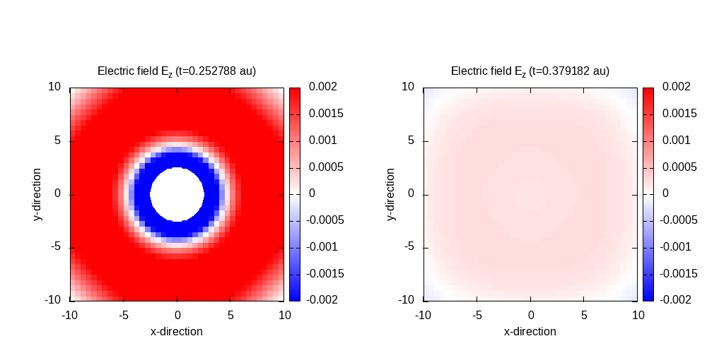
Contour plot of the electric field in z-direction after 120 time steps for
t=0.24 and 180 time steps for t=0.36:
PML boundaries
click for complete input
# ----- Calculation mode and parallelization ------------------------------------------------------

 CalculationMode   = td
 RestartWrite = no
 ExperimentalFeatures = yes

%Systems
  'Maxwell' | maxwell
%

 Maxwell.ParDomains = auto
 Maxwell.ParStates  = no

# ----- Maxwell box variables ---------------------------------------------------------------------

 # free maxwell box limit of 10.0 plus 5.0 for absorbing boundary conditions

 lsize_mx = 15.0
 dx_mx    = 0.5

 Maxwell.BoxShape   = parallelepiped

 %Maxwell.Lsize
  lsize_mx | lsize_mx | lsize_mx
 %

 %Maxwell.Spacing
  dx_mx | dx_mx | dx_mx
 %

# ----- Maxwell calculation variables -------------------------------------------------------------

 MaxwellHamiltonianOperator = faraday_ampere

 %MaxwellBoundaryConditions
  zero | zero | zero
 %

 %MaxwellAbsorbingBoundaries
  cpml | cpml | cpml
 %

 MaxwellABWidth = 5.0
 MaxwellABPMLPower              = 2.0
 MaxwellABPMLReflectionError    = 1e-16

# ----- Output variables --------------------------------------------------------------------------

 OutputFormat = axis_x + axis_y + axis_z + plane_x + plane_y + plane_z


# ----- Maxwell output variables ------------------------------------------------------------------

 %MaxwellOutput
  electric_field
  magnetic_field
  maxwell_energy_density
  trans_electric_field
 %

 MaxwellOutputInterval = 10
 MaxwellTDOutput       = maxwell_energy + maxwell_total_e_field

 %MaxwellFieldsCoordinate
   0.00 | 0.00 | 0.00
 %


# ----- Time step variables -----------------------------------------------------------------------

 TDSystemPropagator = exp_mid
 timestep             = 1 / ( sqrt(c^2/dx_mx^2 + c^2/dx_mx^2 + c^2/dx_mx^2) )
 TDTimeStep           = timestep
 TDPropagationTime    = 180 * timestep

# Maxwell field variables

# ----- External current ------------------------------------------------------------------------

 ExternalCurrent = yes
 t1 = 4 * 5.0 / c
 t2 = 6 * 5.0 / c
 tw = 0.03
 j = 1.0000

 %UserDefinedMaxwellExternalCurrent
   current_td_function | "0" | "0" | "j*exp(-x^2/2)*exp(-y^2/2)*exp(-z^2/2)" | 0 | "env_func_1"
   current_td_function | "0" |" 0" | "j*exp(-x^2/2)*exp(-y^2/2)*exp(-z^2/2)" | 0 | "env_func_2"
 %

 %TDFunctions
   "env_func_1" | tdf_gaussian |  1.0 | tw | t1
   "env_func_2" | tdf_gaussian | -1.0 | tw | t2
 %
We can repeat the simulation using PML absorbing boundaries.
 %MaxwellBoundaryConditions
  zero | zero | zero
 %

 %MaxwellAbsorbingBoundaries
  cpml | cpml | cpml
 %

 MaxwellABWidth = 5.0
 MaxwellABPMLPower              = 2.0
 MaxwellABPMLReflectionError    = 1e-16
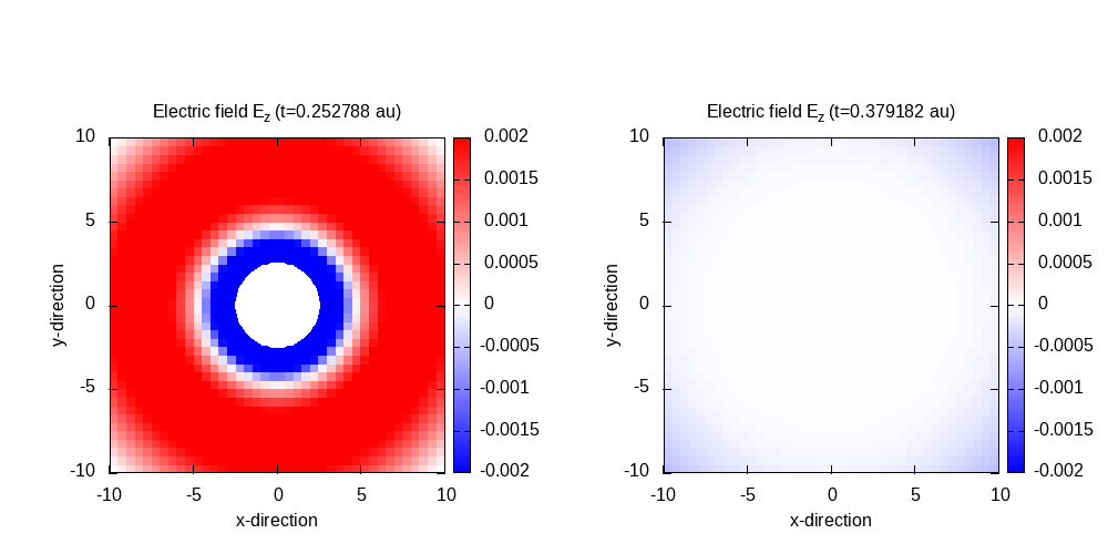
Contour plot of the electric field in z-direction after 120 time steps for
t=0.24 and 180 time steps for t=0.36:
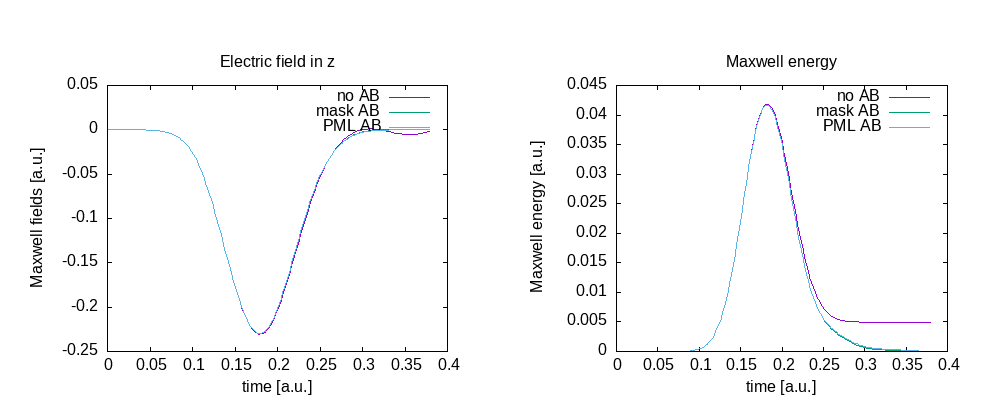
Maxwell fields at the origin and Maxwell energy inside the free Maxwell
propagation region of the simulation box:
Prev
Next