Cosinoidal plane wave in vacuum
Cosinoidal plane wave in vacuum
In this tutorial, we will describe the propagation of a cosinoidal wave in vacuum.
Currently, this run only works with 1 or 2 MPI tasks.
First, define the calculation mode and the parallelization strategy:
# ----- Calculation mode and parallelization ------------------------------------------------------

 CalculationMode                   = td
 ExperimentalFeatures = yes

 %Systems
   'Maxwell' | maxwell
 %

 Maxwell.ParDomains = auto
 Maxwell.ParStates  = no
The total size of the (physical) simulation box is 10.0 x 10.0 x 10.0 Bohr with a spacing of 0.5 Bohr in each direction. As discussed in the section on simulation boxes, also the boundary points have to be accounted for. Hence the total size of the simulation box is chosen to be 12.0 x 12.0 x 12.0 Bohr.
# ----- Maxwell box variables ---------------------------------------------------------------------

 # free maxwell box limit of 10.0 plus 2.0 for the incident wave boundaries with
 # der_order = 4 times dx_mx

 lsize_mx = 12.0
 dx_mx    = 0.5

 Maxwell.BoxShape = parallelepiped

 %Maxwell.Lsize
  lsize_mx | lsize_mx | lsize_mx
 %

 %Maxwell.Spacing
  dx_mx | dx_mx | dx_mx
 %
Since we propagate without a linear medium, we can use the vacuum Maxwell Hamiltonian operator. Derivatives and exponential expansion order are four.
# ----- Maxwell calculation variables -------------------------------------------------------------

 MaxwellHamiltonianOperator = faraday_ampere
The boundary conditions are chosen as plane waves to simulate the incoming wave without any absorption at the boundaries.
 %MaxwellBoundaryConditions
  plane_waves | plane_waves | plane_waves
 %

 %MaxwellAbsorbingBoundaries
  not_absorbing | not_absorbing | not_absorbing
 %
The simulation time step is set to 0.002 and the system propagates to a maximum time step of 200. For each time step, we write an output of the electric and the magnetic field as well as the energy density, the total Maxwell energy.
# ----- Time step variables -----------------------------------------------------------------------

 TDSystemPropagator = exp_mid

 timestep = 1 / ( sqrt(c^2/dx_mx^2 + c^2/dx_mx^2 + c^2/dx_mx^2) )
 TDTimeStep                        = timestep
 TDPropagationTime                 = 150*timestep
The incident cosinoidal plane wave passes the simulation box, where the cosinoidal pulse has a width of 10.0 Bohr, a spatial shift of 25.0 Bohr in the negative x-direction, an amplitude of 0.05 a.u., and a wavelength of 10.0 Bohr.
# ----- Maxwell field variables -------------------------------------------------------------------

 # laser propagates in x direction

 lambda1 = 10.0
 omega1  = 2 * pi * c / lambda1
 k1_x    = omega1 / c
 E1_z    = 0.05
 pw1     = 10.0
 ps1_x   = - 25.0

 %MaxwellIncidentWaves
   plane_wave_mx_function | 0 | 0 | E1_z | "plane_waves_function_1"
 %

 %MaxwellFunctions
   "plane_waves_function_1" | mxf_cosinoidal_wave | k1_x | 0    | 0 | ps1_x | 0     | 0 | pw1
 %
Finally, the output options are set:
# ----- Output variables --------------------------------------------------------------------------

 OutputFormat = plane_x + plane_y + plane_z + axis_x + axis_y + axis_z

# ----- Maxwell output variables ------------------------------------------------------------------

 %MaxwellOutput
  electric_field
  magnetic_field
  maxwell_energy_density
  trans_electric_field
 %

 MaxwellOutputInterval             = 50
 MaxwellTDOutput                   = maxwell_energy + maxwell_total_e_field + maxwell_total_b_field
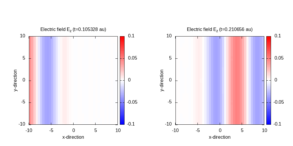
Contour plot of the electric field in z-direction after 50 time steps for t=0.11 and 100 time steps for t=0.21:
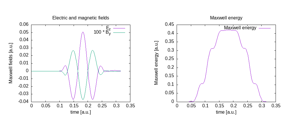
Maxwell fields at the origin and Maxwell energy inside the free Maxwell propagation region of the simulation box: